A Bayesian Workflow for Spatially Correlated Random Effects in On-farm Experiment
(Katia Stefanova, Mark Gibberd, Suman Rakshit)
8/11/22
I’d like to begin by acknowledging the Traditional Owners of the land on which we meet today. I would also like to pay my respects to Elders past and present.
SAGI West Node Research
Analysing Large Strip Experiments: aim is to estimate the spatially-varying treatment effects (e.g., yield response to nitrogen rates) in large paddocks. This may enable the creation of site-specific management zones.
Geographically weighted regression method (published in 2020)
Bayesian analysis framework (published in 2022)
MET framework for categorical variables (submitted)
Deep Gaussian process for spatio-temporal data
On-farm experiments
On-farm experiments
Treatments are applied to adjacent strips to detect spatial variation in treatment response.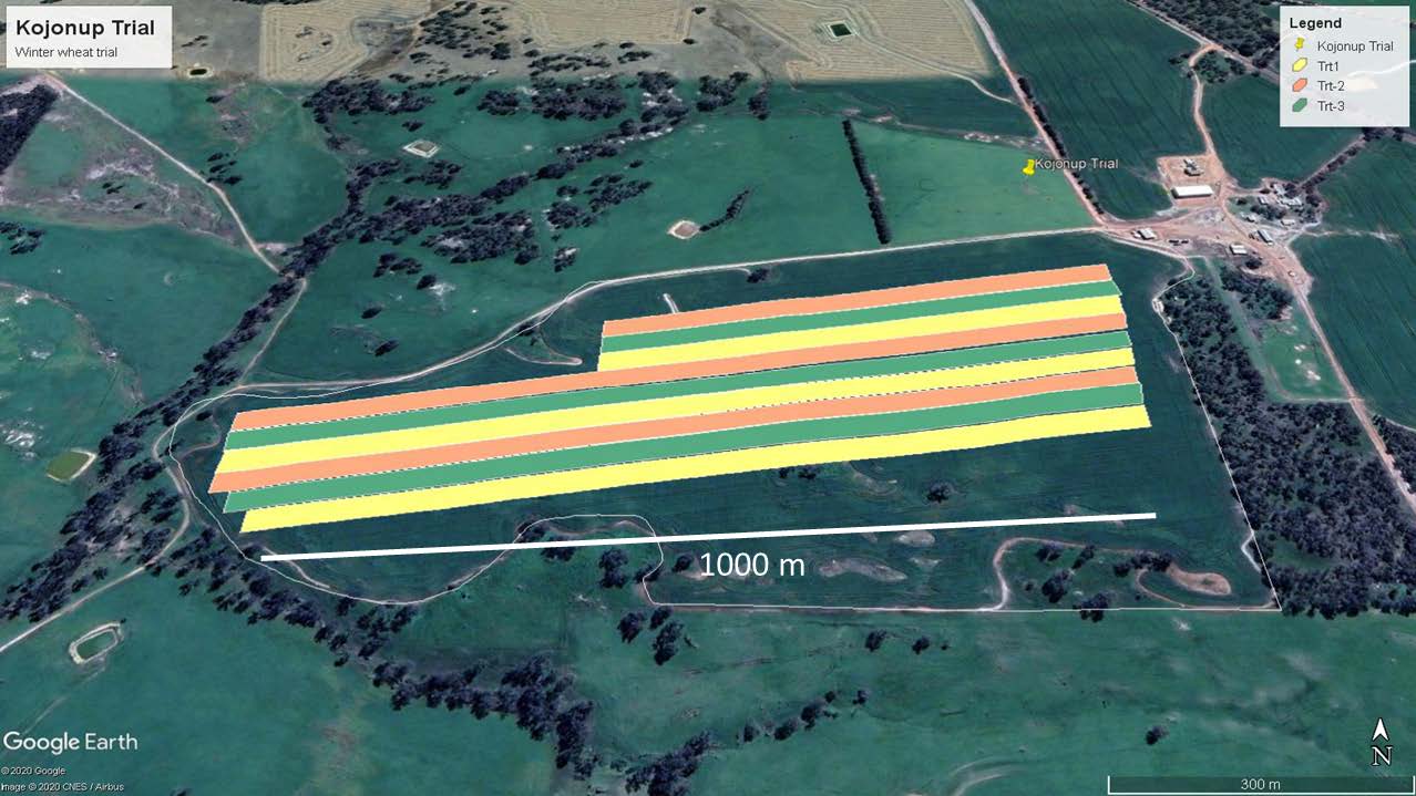
Improve profitability and sustainability
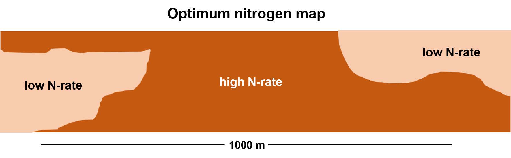
Due to spatial variability, different parts of a field exhibit different yield response to treatments. Some parts may not need high nitrogen rate, and this decreases cost and promotes environmental sustainability.
Identify optimum nitrogen rates
Large scale (strip) trials are needed to identify optimum rates that vary across the field — small plot experiments are ineffective for this purpose.
To generate a spatial map of optimum nitrogen rate, we need to estimate the spatially-varying effects of nitrogen on yield.
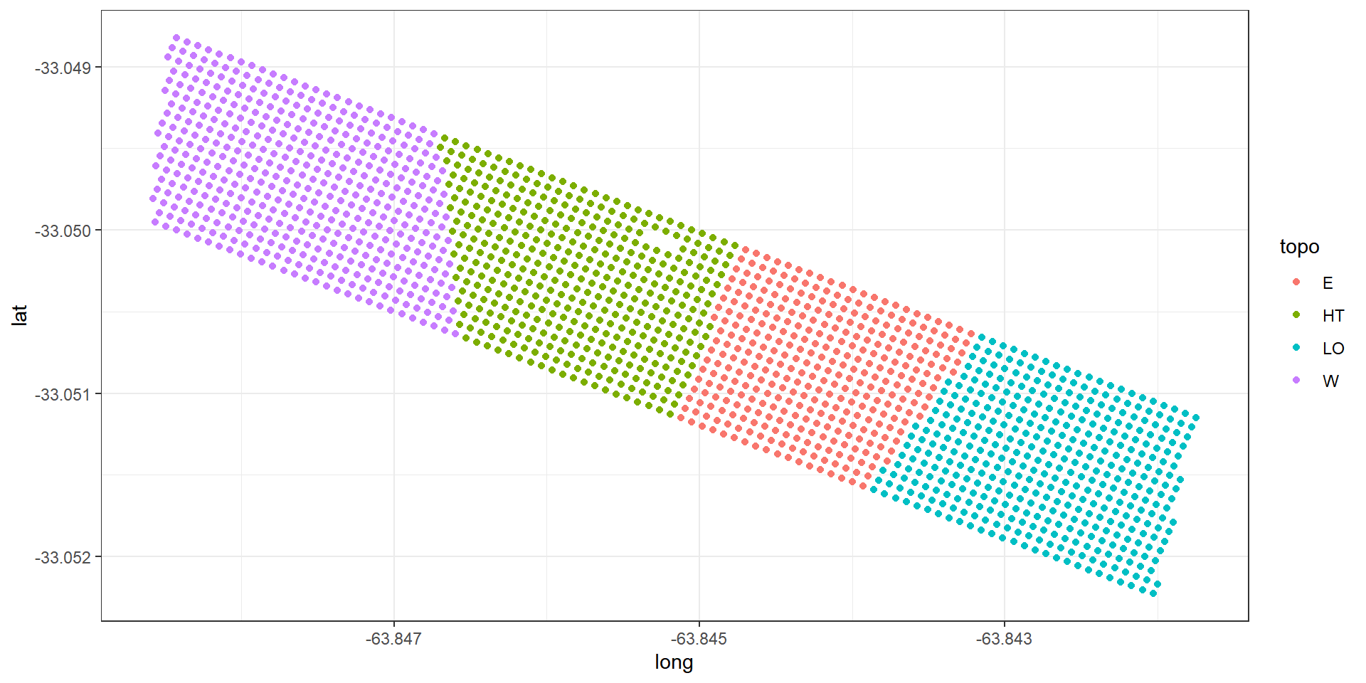
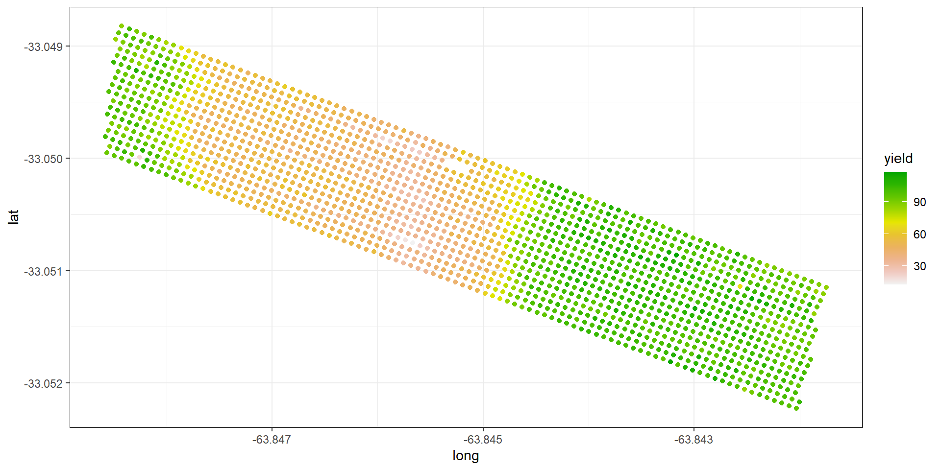
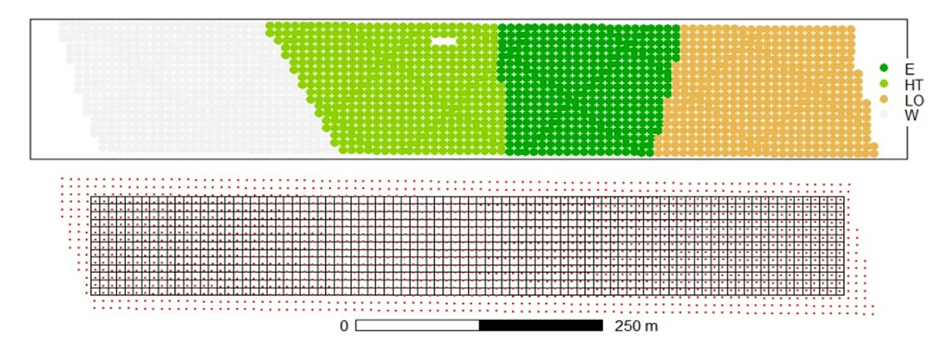
Example: Argentinian corn field experiment
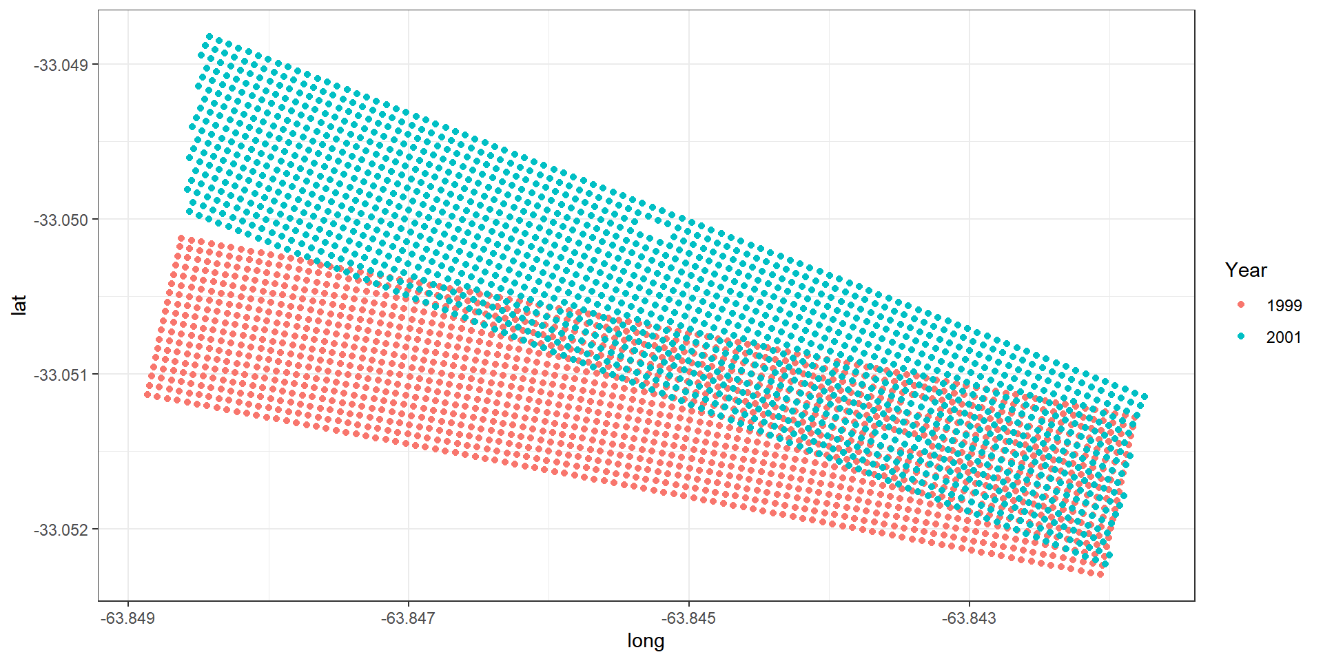
Example: Argentinian corn field experiment
Topographic factor with levels W = West slope, HT = Hilltop, E = East slope, LO = Low East.
Example: Argentinian corn field experiment
Inadequacy of a global model
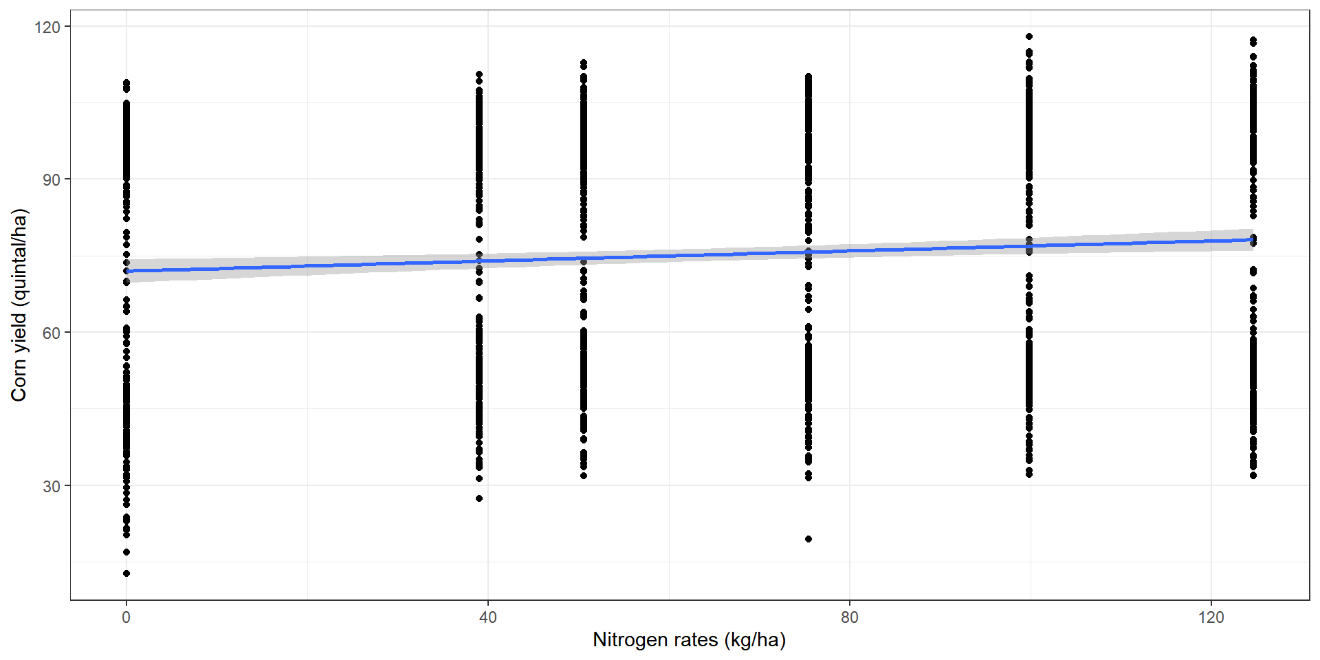
Inadequacy of a global model
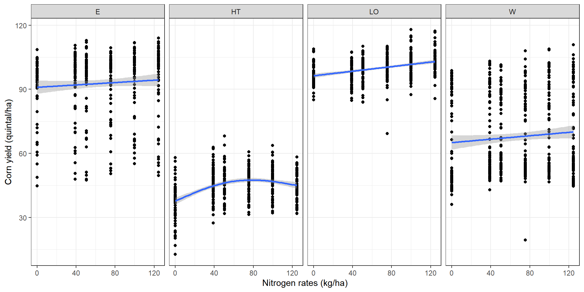
Zone-specific models are limiting
These zonal-boundaries are mostly arbitrary, and do not represent the change points for spatially-varying relationship.
The problem of global model persists within each zone, as we assume that the regression coefficients are constant within each zone. If there is any variation in the spatial relationship within a zone, that would not be captured in a zone-specific regression model.
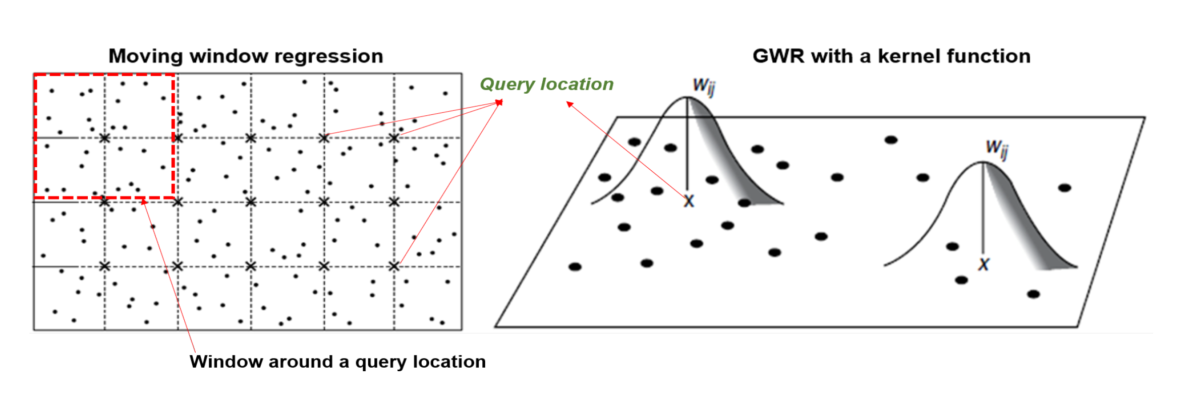
Geographically weighted regression
For constructing the spatial map, we used GWR compute the regression coefficients at regular grid of points covering the study region.
Estimation based on the local-likelihood
Estimate local regression coefficients
Yield prediction with GWR
Bayesian Statistics and Workflow
Why Bayesian?
Liear mixed model notation
A linear mixed effects model for
Liear mixed model notation
Therefore,
Bayesian hierarchical model
At location
Particular model
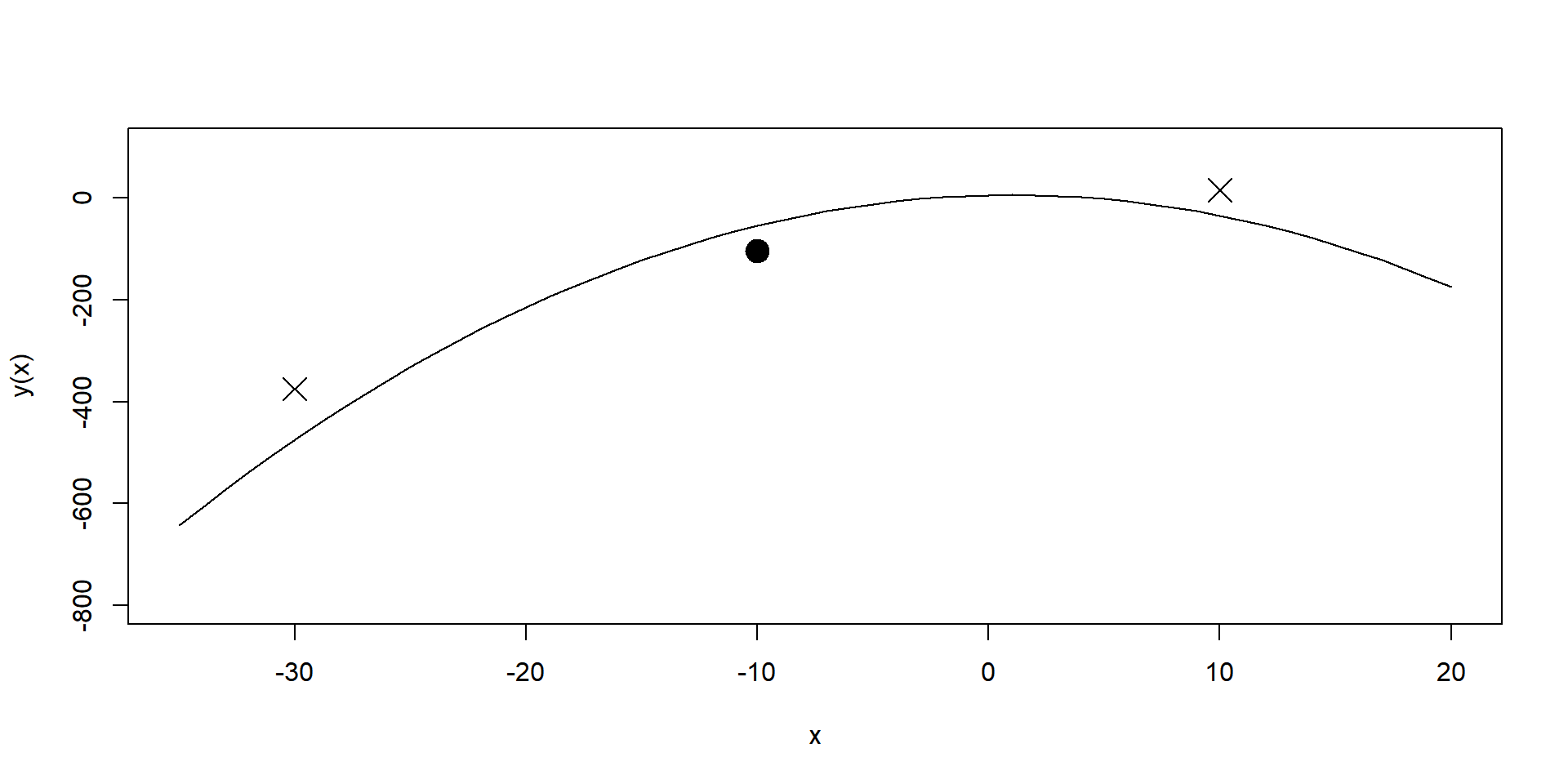
A regression model of particular interest is the quadratic response model. The term associated with the global effects would take the form:
Spatially correlated random parameters
For all
Why use spatially correlated Σu ?
- Only a single treatment is directly observed in any one position.
Why use spatially correlated Σu ?
The spatial model allows the exploiting of information from neighboring positions with other treatments (Piepho et al. (2011)).
Bayesian workflow
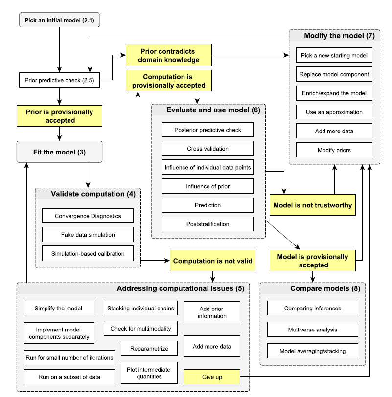
Bayesian process
Suppose
Posterior distribution
In order to estimate
Likelihood
We obtain for multivariate Gaussian distribution
Prior specification
Usually, if nothing is known from earlier studies, we can use a flat non-informative prior
p(θ)(∝constant) , also called an “improper prior” (Gelman et al. (2006)).In many circumstances, a Cauchy or Gamma prior is a reasonable candidate for regression coefficients. Inverse Wishart (IW) or inverse Gamma as the prior distribution for the standard deviation parameter of a hierarchical model.
Gelman et al. (2006), Gelman, Simpson, and Betancourt (2017) suggested weakly informative priors for variance parameters for Bayesian analyses of hierarchical linear model
Prior specification
To specify a prior distribution for the parameters associated with the variance-covariance matrix
Prior specification
For the matrix
LKJ Prior

Predictive distribution
The predictive distribution for a new query location
Posterior sampling with Markov chains
For high-dimensional problems, the most widely used random sampling methods are Markov chain Monte Carlo methods.
Posterior sampling with Markov chains
However, simple Metropolis algorithms and Gibbs sampling algorithms, although widely used, perform poorly because they explore the space by a slow random walk (MacKay, Mac Kay, et al. (2003)).
Random walk Metropolis-Hastings
source:https://github.com/chi-feng
Hamiltonian Monte Carlo (HMC)
Hamiltonian Monte Carlo (HMC) (Brooks et al. (2011), Duane et al. (1987)) is an efficient Markov chain Monte Carlo (MCMC) method that overcomes the inefficiency associated with the random walk and with the sensitivity to correlated parameters.
An important step in HMC is the drawing of a set of auxiliary momentum variables
r={r1,…,rd} , independently from the standard normal distribution for each parameter in the setθ={θ1,…,θd} . The joint density functionf(θ,r) ofθ andr is given bywheref(θ,r)∝exp{L(θ)−K(r)}=exp{−H(θ,r)}, H(θ,r) is the Hamiltonian system dynamics (HSD) equation with potential energyL(θ) and kinetic energyK(r) .
Hamiltonian Monte Carlo (HMC)
The HSD is numerically approximated in discrete time space with the leapfrog method to maintain the total energy when a new sample
(θ∗,r∗) is drawn.The leapfrog method requires two parameters: (i) a step size
ϵ , representing the distance between two consecutive draws, and (ii) a desired number of stepsL , required to complete the process. A new sample is accepted with the probabilityα=min{1,f(θ∗,r∗)f(θ,r)}.
Hamiltonian Monte Carlo (HMC)
source:https://github.com/chi-feng
Problems with HMC
HMC is highly sensitive to the choice of
source:https://github.com/chi-feng
No-U-Turn Sampler (NUTS)
No-U-Turn Sampler (NUTS) determines the step size adaptively during the warm-up (burn-in) phase to a target acceptance rate and uses it then for all sampling iterations (Hoffman and Gelman (2014), Monnahan, Thorson, and Branch (2017)).
The NUTS also eliminates the need to specify a value of
No-U-Turn Sampler (NUTS)
The slice sampling generates a finite set of samples of the form
No-U-Turn Sampler (NUTS)
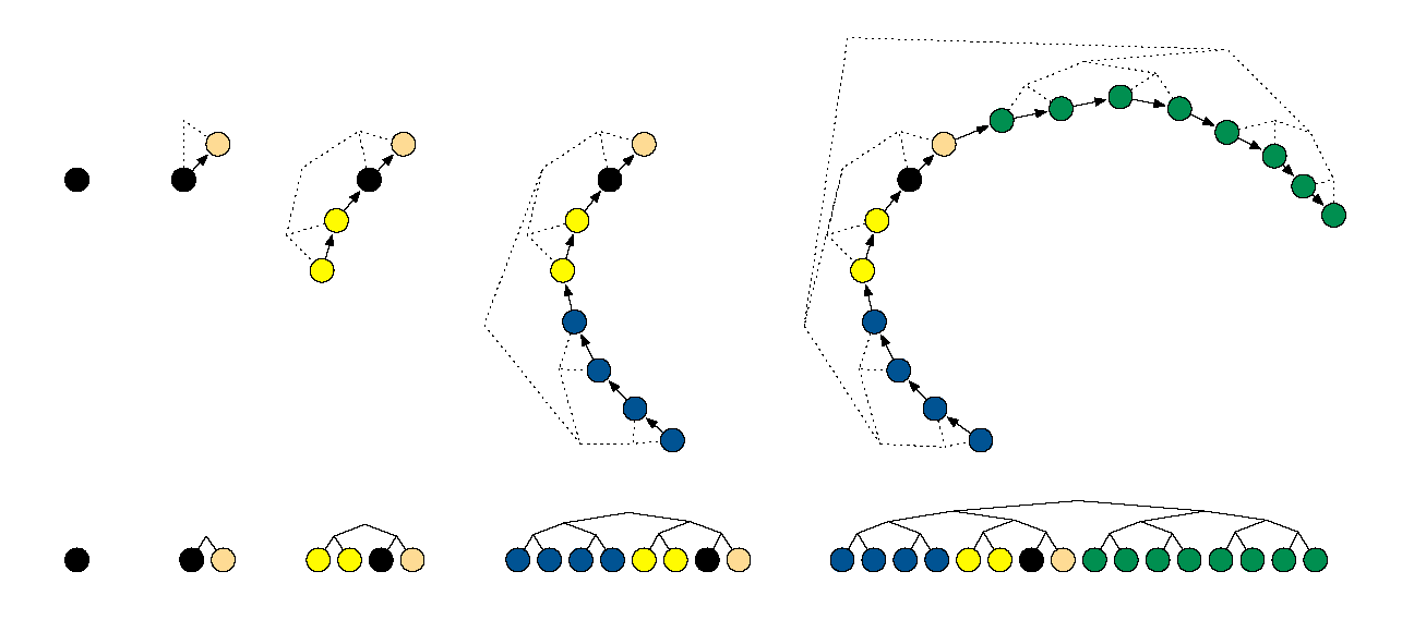
Example of building a binary tree via repeated doubling (Hoffman and Gelman (2014)).
No-U-Turn Sampler (NUTS)
source:https://github.com/chi-feng
No-U-Turn Sampler (NUTS)
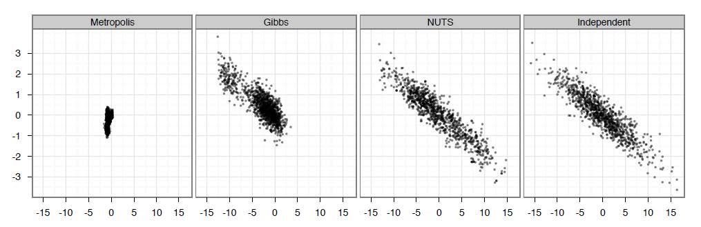
Samples generated by random-walk Metropolis, Gibbs sampling, and NUTS. (Hoffman and Gelman (2014))
Posterior predictive checking
The posterior predictive (PP) checking uses the posterior distribution of the model parameters to regenerate the observations.
Let
Leave-one-out (LOO) cross validation
In Bayesian statistics, the expected
Bürkner, Gabry, and Vehtari (2021) proposed approximated LOO CV, which uses only a single model fit and calculating the pointwise
Pareto-smoothed importance-sampling (PSIS)
The LOO estimate is improved by using Pareto smoothed importance sampling which applies a smoothing procedure to the importance weights (Vehtari, Gelman, and Gabry (2017)).
The PSIS-LOO-CV estimate is computed taking a weighted sum over all
Pareto-smoothed importance-sampling (PSIS)
The estimated shape parameter
If
k<12 , the variance of the raw importance ratios is finite, the central limit theorem holds, and the estimate converges quickly.If
12<k<1 , the variance of the raw importance ratios is infinite but the mean exists, the generalized central limit theorem for stable distributions holds, and the convergence of the estimate is slower. The variance of the PSIS estimate is finite but may be large.If
k>1 , the variance and the mean of the raw ratios distribution do not exist. The variance of the PSIS estimate is finite but may be large.
Bayesian R2
The Bayesian
- It should not be interpreted solely if the model has a large number of bad Pareto
k^ values, i.e., values greater than 0.7 or, even worse, greater than 1.
Las Rosas data
Las Rosas data
To obtain the map of locally varying optimal input rates, we specified a quadratic regression model, in which the corn yield is modelled as a quadratic function of the nitrogen rate. The optimal treatment can be determined by estimating the coefficients of the quadratic regression model at each grid point.
| Model 1 | Model 2 | Model 3 | Model 4 | |
|---|---|---|---|---|
| Spatial correlation | No | Yes | No | Yes |
| Distribution | Gaussian | Gaussian | Student- |
Student- |
RStan
RStan is the R interface to the Stan C++ package. RStan provides
- full Bayesian inference using the No-U-Turn sampler (NUTS), a variant of Hamiltonian Monte Carlo (HMC)
- approximate Bayesian inference using automatic differentiation variational inference (ADVI)
- penalized maximum likelihood estimation using L-BFGS optimization
RStan
functions {
  matrix chol_AR_matrix(real rho,int d){
    matrix[d,d] MatAR;
    MatAR = rep_matrix(0,d,d);
    for(i in 1:d){
      for(j in i:d){
        if(j>=i && i==1) MatAR[j,i] = rho^(j-1);
        else if(i>=2 && j>=i) MatAR[j,i] = rho^(j-i)*sqrt(1-rho^2);
      }
    }
    return MatAR;
  }
}
data {
  int<lower=1> N;
  vector[N] Y;
  int<lower=1> K;
  matrix[N, K] X;
  int<lower=1> N_1;
  int<lower=1> M_1;
  int<lower=1> J_1[N];
  vector[N] Z_1_1;
  int nrow;
  int ncol;
}
transformed data {
  int Kc = K - 1;
  matrix[N, Kc] Xc;
  vector[Kc] means_X;
  for (i in 2:K) {
    means_X[i - 1] = mean(X[, i]);
    Xc[, i - 1] = X[, i] - means_X[i - 1];
  }
}
parameters {
  vector[Kc] b;
  real Intercept;
  real<lower=0> sigma;
  vector<lower=0>[M_1] sd_1;
  vector[N_1] z_1[M_1];
  matrix[ncol, nrow] z_2;
  real<lower=0,upper=1> rho_r;
  real<lower=0,upper=1> rho_c;
}
transformed parameters {
  vector[N_1] r_1_1;
  vector[N] Sig;
  r_1_1 = (sd_1[1] * (z_1[1]));
  Sig = sigma * to_vector(chol_AR_matrix(rho_c,ncol) * z_2 * chol_AR_matrix(rho_r,nrow)"'");
}
model {
  vector[N] mu = Intercept + rep_vector(0.0, N);
  for (n in 1:N) {
    mu[n] += r_1_1[J_1[n]] * Z_1_1[n] + Sig[n];
  }
  target += normal_id_glm_lpdf(Y | Xc, mu, b, sigma);
  // prior
  target += student_t_lpdf(Intercept | 3, 84.7, 31.3);
  target += student_t_lpdf(sigma | 3, 0, 31.3)
    - 1 * student_t_lccdf(0 | 3, 0, 31.3);
  target += student_t_lpdf(sd_1 | 3, 0, 31.3)
    - 1 * student_t_lccdf(0 | 3, 0, 31.3);
  target += std_normal_lpdf(z_1[1]);
  target += std_normal_lpdf(to_vector(z_2));
  target += uniform_lpdf(rho_r | 0,1) + uniform_lpdf(rho_c | 0,1);
}
generated quantities {
  vector[N] log_lik;
  vector[N] y_rep;
  vector[N] mu = Intercept + Xc * b;
  real b_Intercept = Intercept - dot_product(means_X, b);
  for (n in 1:N) {
    mu[n] += r_1_1[J_1[n]] * Z_1_1[n] + Sig[n];
    log_lik[n] = normal_lpdf(Y[n] | mu[n], 1);
  }
}
RStan
Other packages:
brms (R)
rstanarm (R)
glmer2stan (R)
PyStan (Python stan)
Stan.jl (Julia stan)
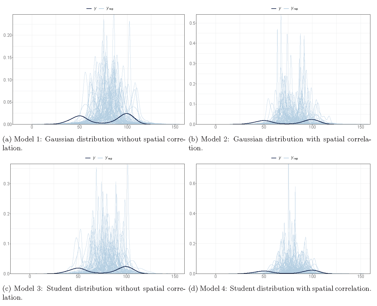
Prior predictive simulations
| Model 1 | Model 2 | Model 3 | Model 4 | |
|---|---|---|---|---|
|
|
|
|||
|
|
|
|||
|
|
|
|||
|
|
|
|||
|
|
|
|||
|
|
|
|||
|
|
|
|||
|
|
— | LKJcorr(1) | — | LKJcorr(1) |
|
|
— |
|
— |
|
|
|
— |
|
— |
|
|
|
— | — |
|
|
Prior predictive simulations
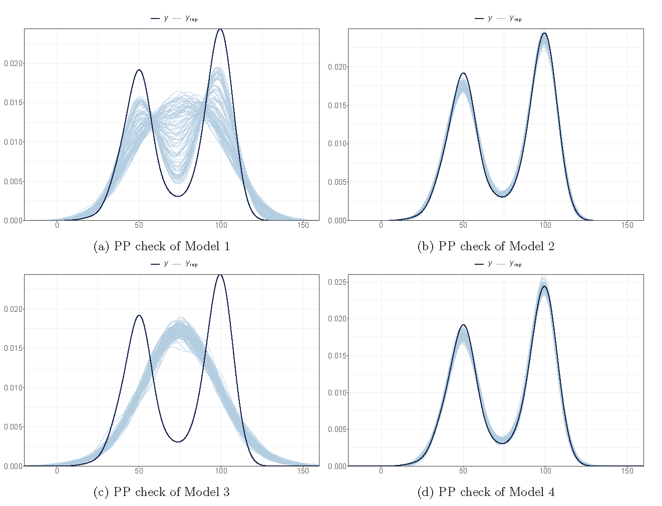
Posterior checking (fitting)
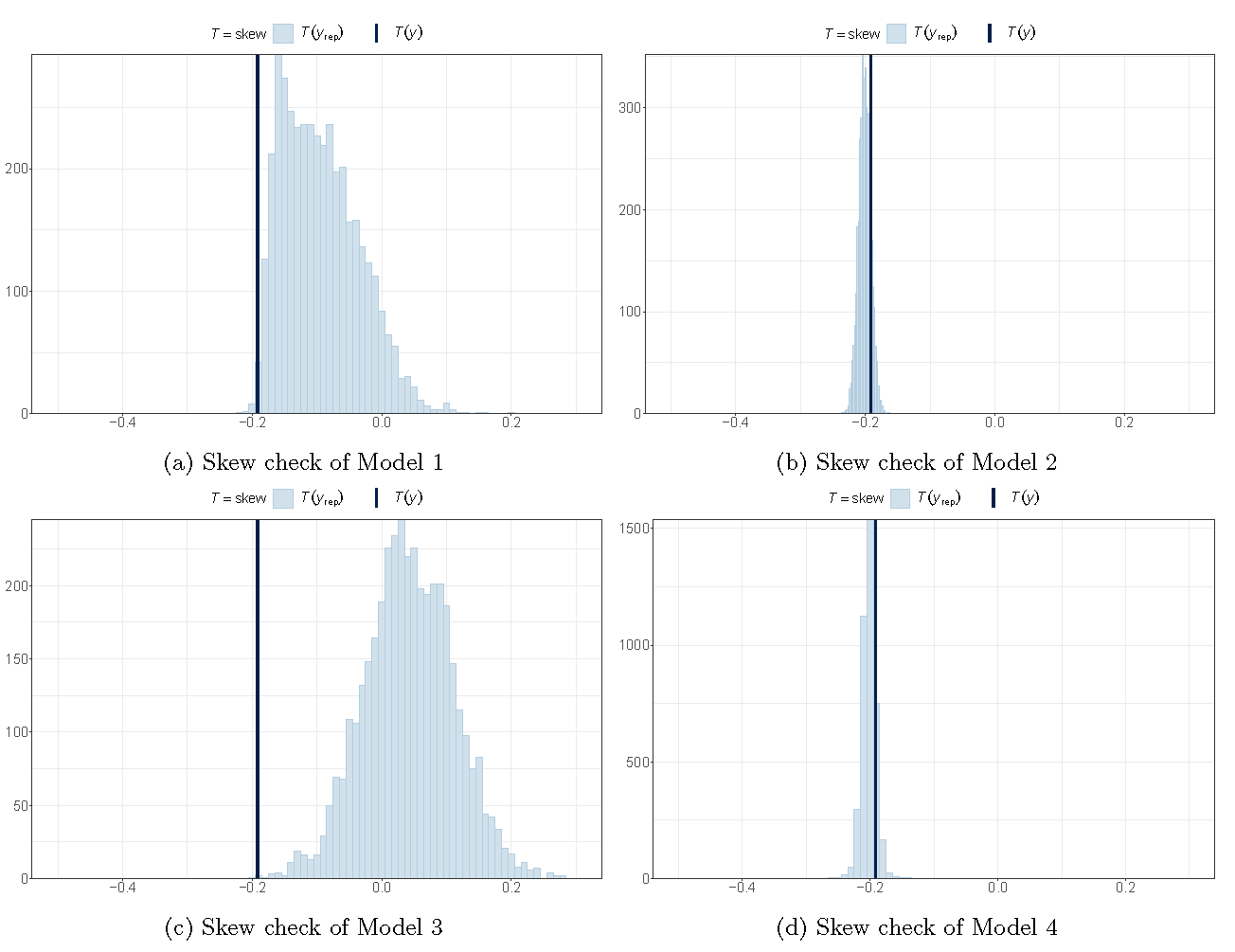
Posterior checking (skewness)
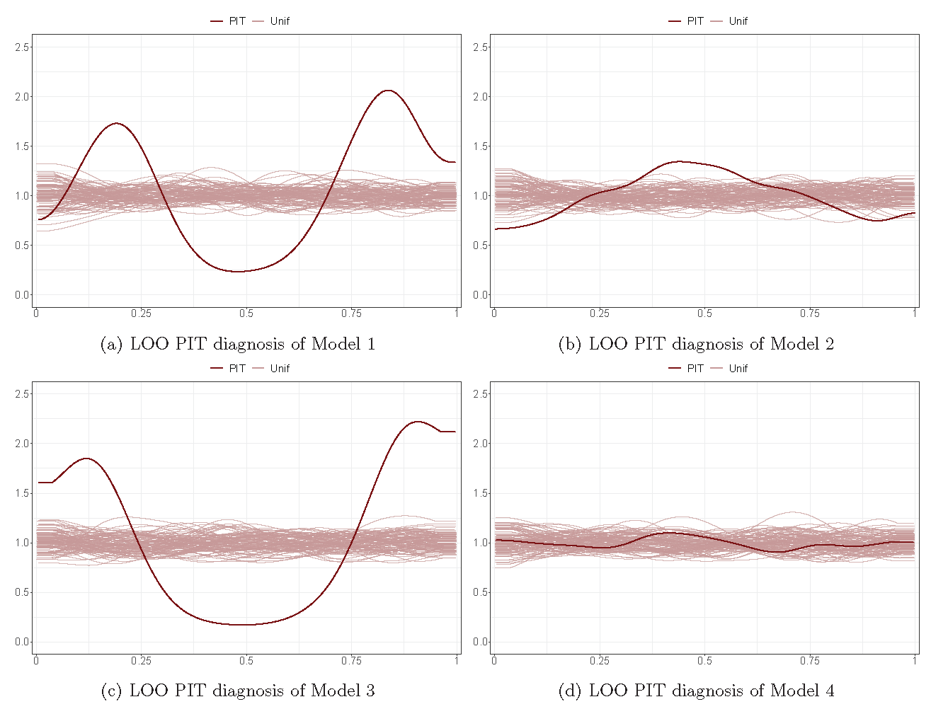
Posterior checking (LOO PIT)
Pareto k^
| Model 1 | Model 2 | Model 3 | Model 4 | |||||||||
|---|---|---|---|---|---|---|---|---|---|---|---|---|
| Count | Per | M.Eff | Count | Per | M.Eff | Count | Per | M.Eff | Count | Per | M.Eff | |
| (-Inf, 0.5] (good) | 28 | 1.7% | 457 | 1585 | 94.7% | 432 | 1474 | 88.1% | 494 | 1672 | 99.9% | 868 |
| (0.5, 0.7] (ok)(good) | 372 | 22.2% | 112 | 83 | 5.0% | 103 | 176 | 10.5% | 254 | 2 | 0.1% | 1733 |
| (0.7, 1] (bad) | 1138 | 68.0% | 18 | 4 | 0.2% | 70 | 24 | 1.4% | 170 | 0 | 0.0% | 0 |
| (1, Inf) (very bad) | 136 | 8.1% | 8 | 2 | 0.1% | 4 | 0 | 0.0% | 0 | 0 | 0.0% | 0 |
Model evaluation
| Model 1 | Model 2 | Model 3 | Model 4 | |||||
|---|---|---|---|---|---|---|---|---|
| Estimate | SE | Estimate | SE | Estimate | SE | Estimate | SE | |
| elpd | -7236.2 | 13.4 | -4945.2 | 134.8 | -7848.4 | 17.1 | -4734.3 | 38.3 |
| ploo | 1487.1 | 11.7 | 341.8 | 41.3 | 241.2 | 6.8 | 516.1 | 10.5 |
| looic | 14472.5 | 26.7 | 9890.4 | 269.6 | 15696.8 | 34.3 | 9468.7 | 76.7 |
| Median | CI | Median | CI | Median | CI | Median | CI | |
|---|---|---|---|---|---|---|---|---|
|
Bayesian |
0.842 |
0.563 |
0.974 |
0.972 |
0.190 |
0.135 |
0.989 |
0.987 |
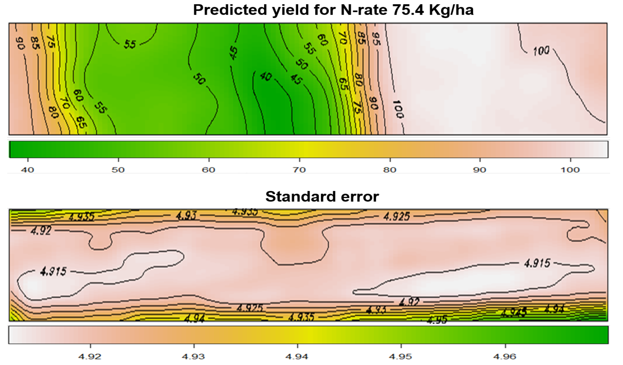
Results
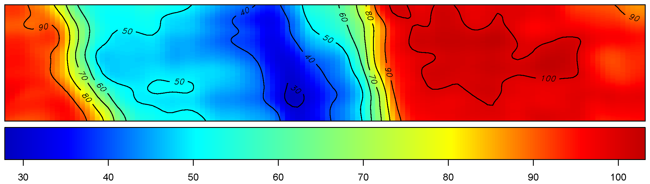
Yield
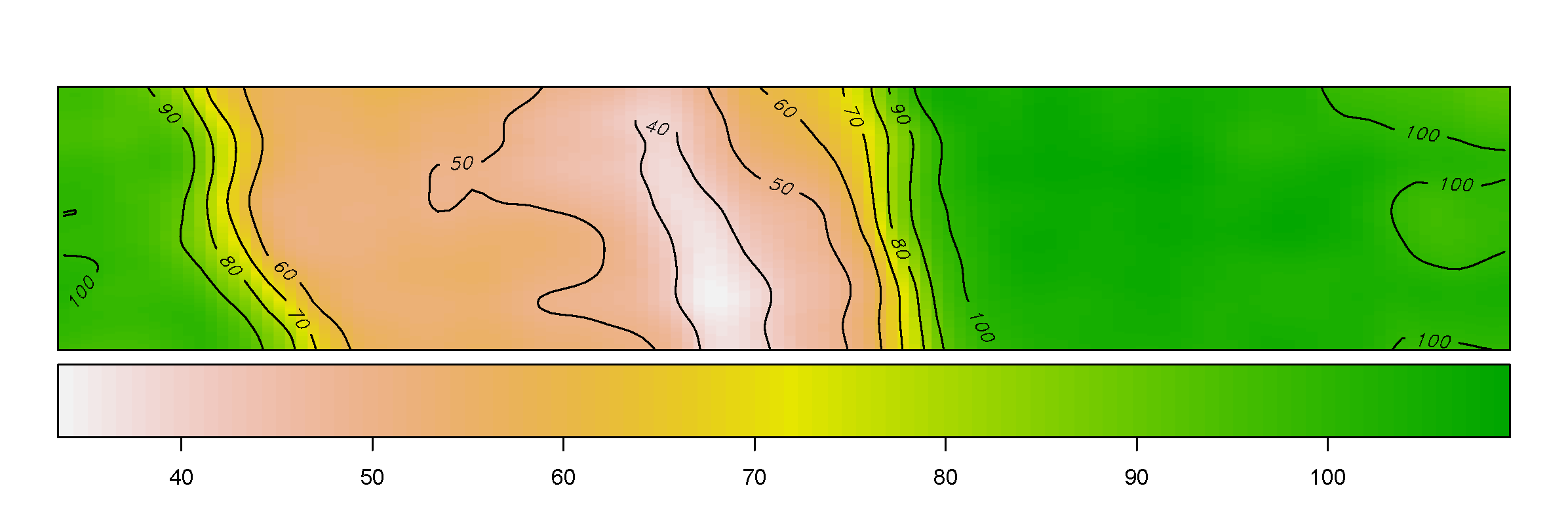
The figure depicts the map of the estimated yield corresponding to the spatially-varying adjusted optimal treatment rates across the field.
Compare with GWR
| GWR | Bayesian | |
|---|---|---|
| Inference | with neighbouring data | with all data |
| Initialisation | bandwidth selection | prior specification |
| Objective | local log-likelihood | global log-likelihood |
| Evaluation | credible intervals | |
| PP check and LOO PIT | ||
| Pareto |
||
| Bayesian |
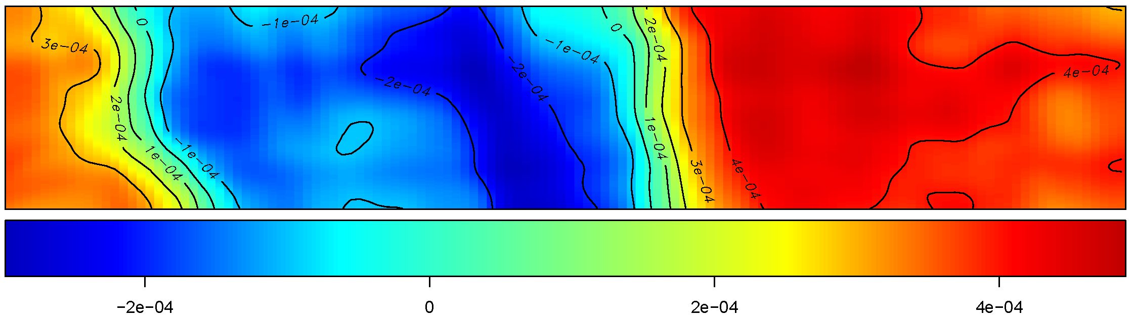
Further application of BHM and GWR
Two types of large-strip trial design

Response

Spatial correlation
For the variance-covariance of the random effects,
Results

Results

Take-home message
- Large strip trials
- Visualization: prior checking, posterior checking
- Diagnosis and evaluation: LOO, PIT, Parote
k ,R2 - NUTS: rstan
- A systematic design is suprior to a randomised design in some way
References
Thank you.