Proving the Superiority of Systematic Designs in On-Farm Trials

Puzzles

The first piece: GWR

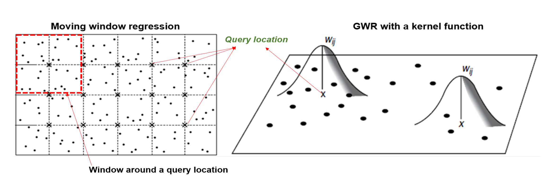
For constructing the spatial map, we used Geographically Weighted Regression (GWR) compute the regression coefficients at regular grid of points covering the study region (Rakshit et al. (2020)).

Estimation based on the local-likelihood
Estimate local regression coefficients

source: Fotheringham, Brunsdon, and Charlton (2003)

The second piece: BHM

The Bayesian hierarchical model (BHM) is a powerful tool for spatial data analysis.
It is a flexible approach to model spatially correlated data.
The BHM is used to estimate the regression coefficients at all grid points simultaneously (Cao et al. (2022)).
The BHM is a complementary approach to GWR.

In GWR, the results crucially depends on the bandwidth of the selected kernel function. Although an appropriate bandwidth can be selected using spatial cross validation, it is computationally challenging for large data sets. To estimate the regression parameters for a query location, the neighbouring observations are given more weight than the distant ones in GWR. On the contrary, the proposed Bayesian approach uses all data in one go to produce estimates for all grid point, based on a spatial variance matrix defined for the entire field. The Bayesian inference is affected by the choice of priors and the likelihood. However, the influence of the prior reduces if the amount of data increases. The Bayesian approach in general is more flexible than GWR, as it can be easily extended and applied broadly to other applications.

The second piece: BHM

At location $s_i$ , the model is written as

\begin{aligned} y (s_{i}) = \sum_{m = 1}^{l} b_{m} x_{m} (s_{i}) + \sum_{j = 1}^{h} u_{j} (s_{i}) z_{j} (s_{i}) + e (s_{i}), \\ u_{i} ∣ θ_{u} \sim N (0, V_{u} (θ_{u})), \\ e (s_{i}) ∣ σ_{e} \sim N (0, σ_{e}^{2}) . \end{aligned}

$\begin{split} & y(s_i) = \sum_{m=1}^{l}b_m x_m(s_i) + \sum_{j=1}^{h}u_j(s_i)z_j(s_i)+e(s_i), \\ & \boldsymbol{u}_i \mid \theta_u \sim \N(0,V_u(\theta_u)), \\ & e(s_i) \mid \sigma_e \sim \N(0,\sigma_e^2). \end{split}$

In matrix notation,

Y \sim N (X b + Z u, e) .

$\boldsymbol{Y} \sim \N\left(\boldsymbol{X}\boldsymbol{b} + \boldsymbol{Z}\boldsymbol{u}, \boldsymbol{e}\right).$

Spatially correlated random parameters

For all $\bm{u} = \{\bm{u}_1,\ldots,\bm{u}_n\}$ , the variance is

Σ_{u} = I_{n} \otimes V_{u} .

$\Sigma_u = I_n \otimes V_u.$ Or

Σ_{u} = V_{s} \otimes V_{u} .

$\Sigma_u = V_s \otimes V_u.$

$V_s$ can be $\AR\otimes\AR$ for regular grid data or Matérn covariance function for irregular grid data.

Spatially correlated random parameters

Using this structure is because that only a single treatment is directly observed in any one position.

The spatial model allows the exploiting of information from neighbouring positions with other treatments (Piepho et al. (2011)).

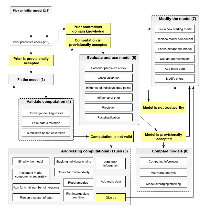
Bayesian workflow

Results

Maps for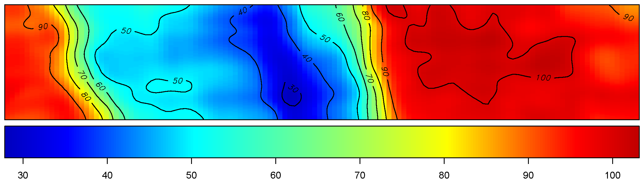

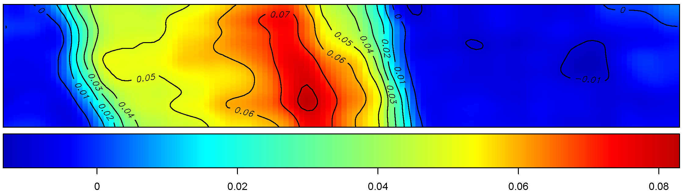
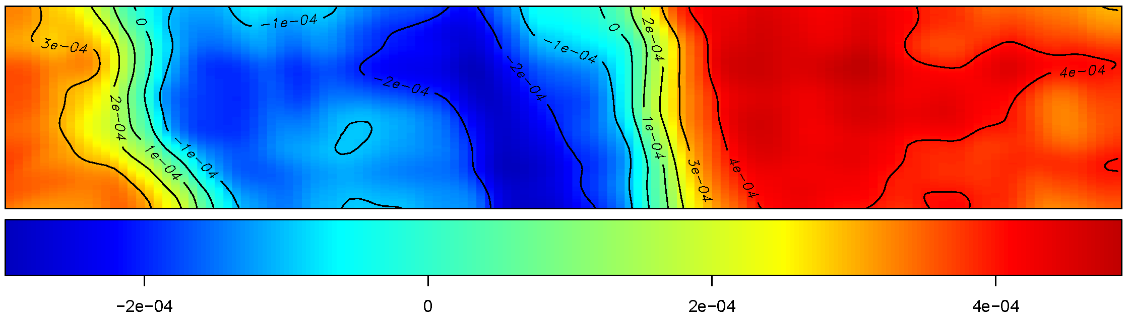
{\hat{β}}_{0}

$\hat{\beta}_0$ ,

{\hat{β}}_{1}

$\hat{\beta}_1$ , and

{\hat{β}}_{2}

$\hat{\beta}_2$ .

Putting two pieces together

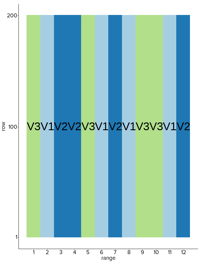
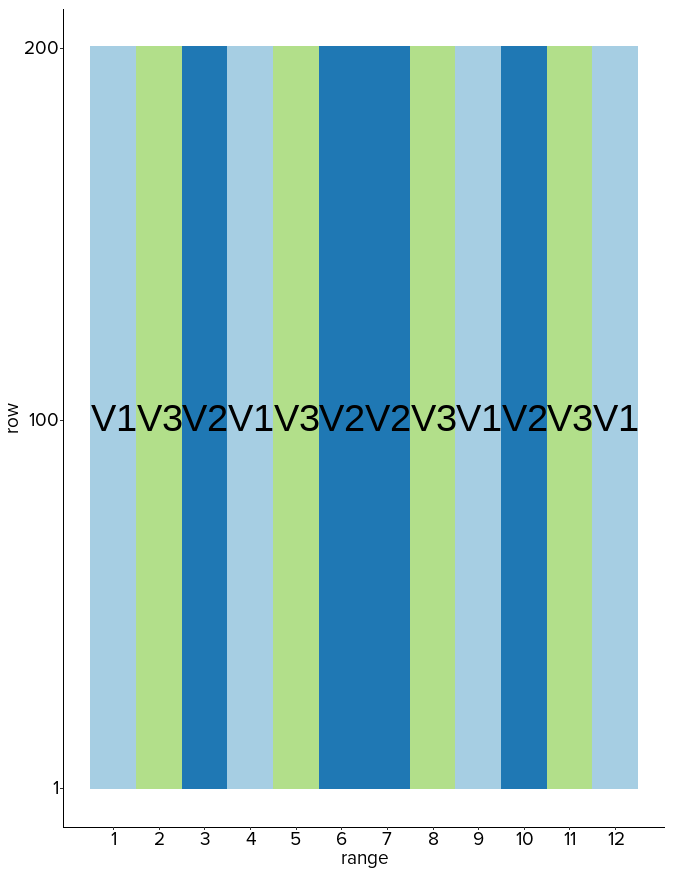
The third piece: trial designs

BHM to generate synthetic OFE data and we know the true values $b$ and $u$ .
GWR to fit the data and estimate coefficients $\hat{\beta}$ .
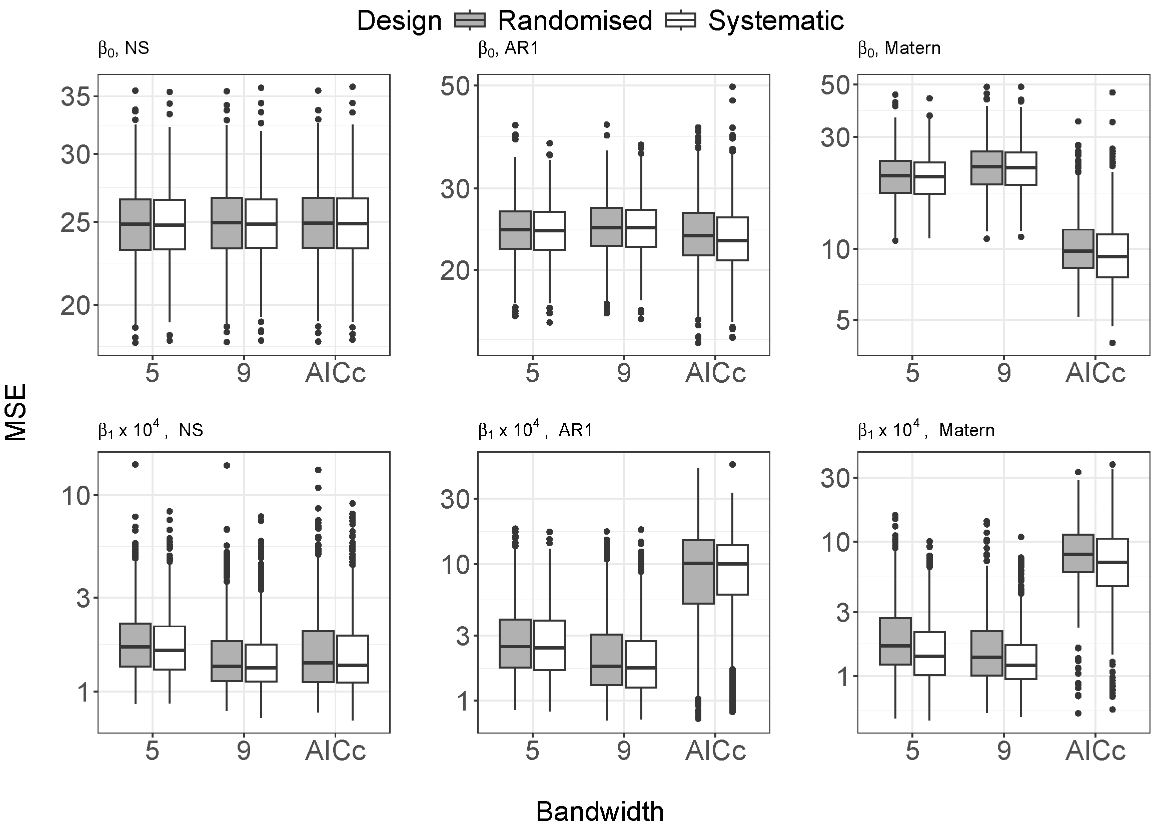
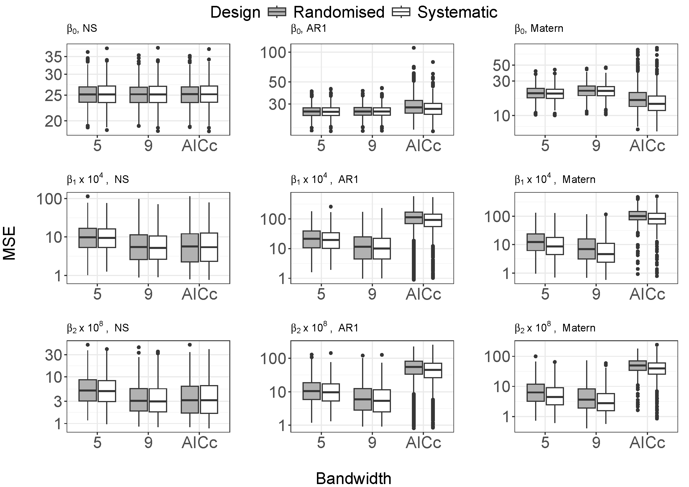
Evaluation: Mean Squared Errors
${MSE}_{j} = \frac{1}{n} \sum_{i = 1}^{n} {({\hat{β}}_{i j} - (b_{i} + u_{i}))}^{2}$ $\mbox{MSE}_j = \frac{1}{n}\sum_{i=1}^n \left(\hat{\beta}_{ij}-(b_i+u_i)\right)^2$ where $j = 0,1$ or $j = 0,1,2$ (Cao et al. (2024)).

Different designs

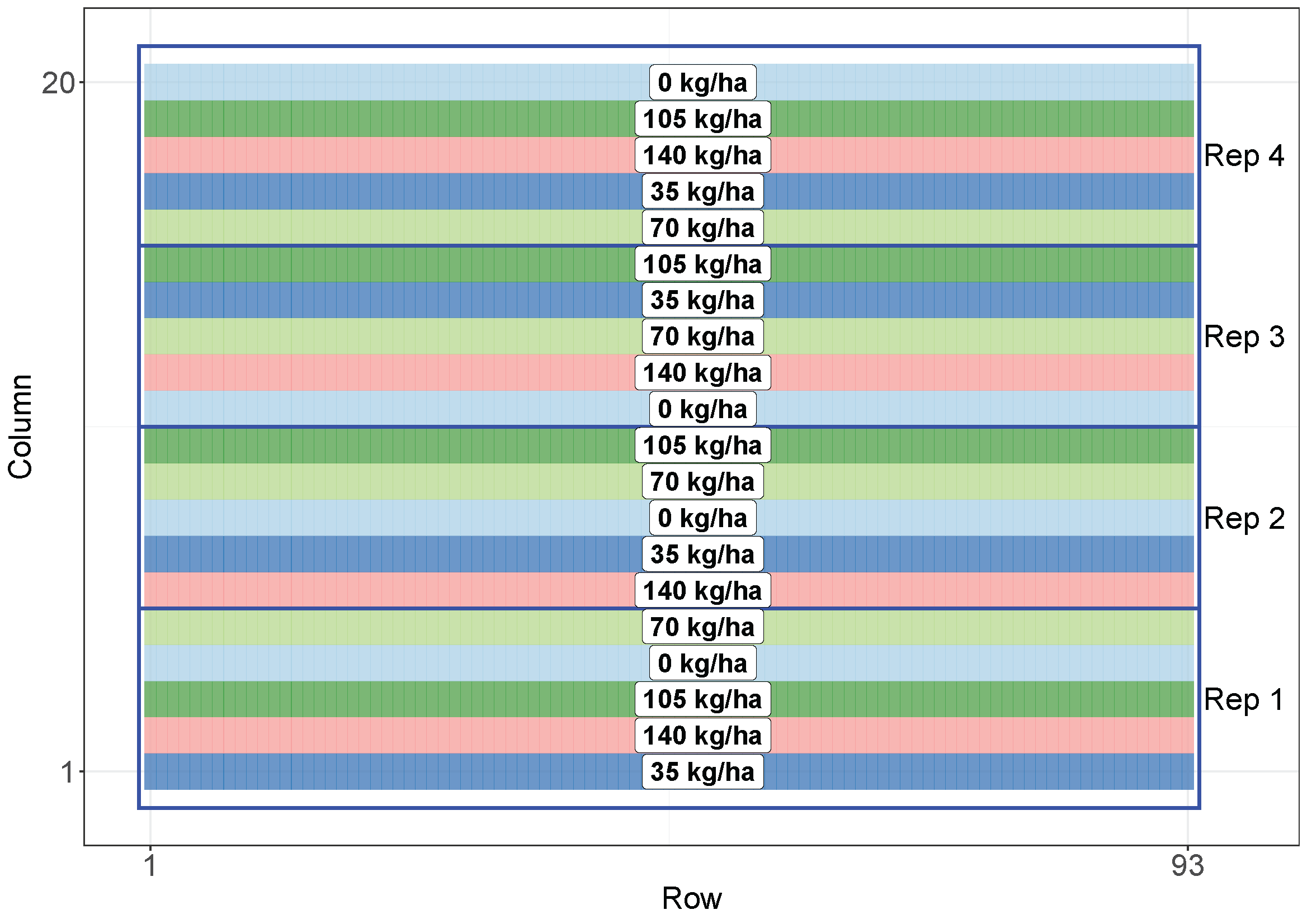
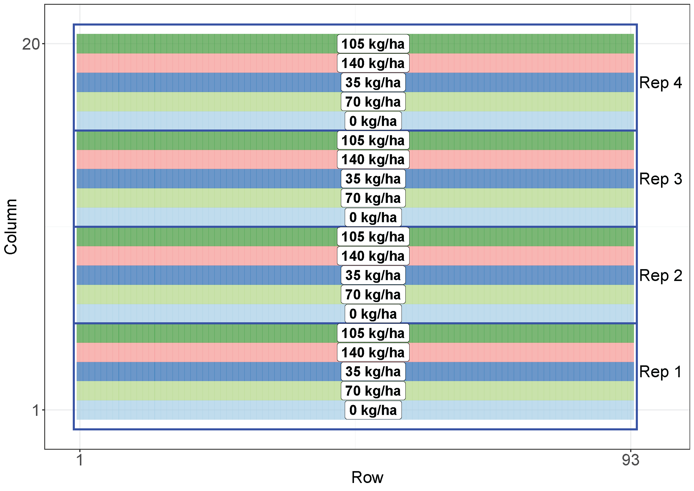
5 treatments, 4 replicates, 93 rows $\times$ 20 ranges

Other factors

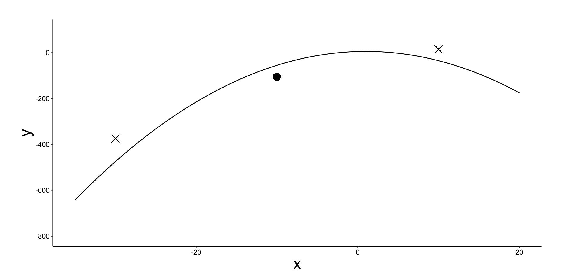
Response types: linear and quadratic
${\begin{cases} Linear & y_{i} = b_{0} + u_{0 i} + (b_{1} + u_{1 i}) N_{i} + e_{i} \\ Quadratic & y_{i} = b_{0} + u_{0 i} + (b_{1} + u_{1 i}) N_{i} + (b_{2} + u_{2 i}) N_{i}^{2} + e_{i} \end{cases},$ $\begin{equation} \begin{cases} % \text{Linear} &y_i = b_0 + b_1N_i + u_{0i} + u_{1i}N_i + e_i \\ \text{Linear} &y_i = b_0 + u_{0i} + (b_1 + u_{1i})N_i + e_i \\ % \text{Quadratic} &y_i = b_0 + b_1N_i + b_2N_i^2 + u_{0i} + u_{1i}N_i + u_{2i}N_i^2 + e_i \text{Quadratic} &y_i = b_0 + u_{0i} + (b_1 + u_{1i})N_i + (b_2 + u_{2i})N_i^2 + e_i \end{cases}, \end{equation}$
Variance-covariance of the random effects, $V_s = I$ , $V_s = \AR(\rho_c)\otimes \AR(\rho_r)$ and Matérn covariance
$V_{s} (d) = σ^{2} \frac{2^{1 - ν}}{Γ (ν)} {(\sqrt{2 ν} \frac{d}{r})}^{ν} K_{ν} (\sqrt{2 ν} \frac{d}{r}) .$ $\begin{equation}\label{eq:matcov} V_s(d) = \sigma^2 \frac{2^{1-\nu}}{\Gamma(\nu)} \left( \sqrt{2\nu} \frac{d}{r}\right)^\nu K_\nu\left( \sqrt{2\nu} \frac{d}{r}\right). \end{equation}$
Bandwidth selection
Correlation intensity

Results

Putting three pieces together

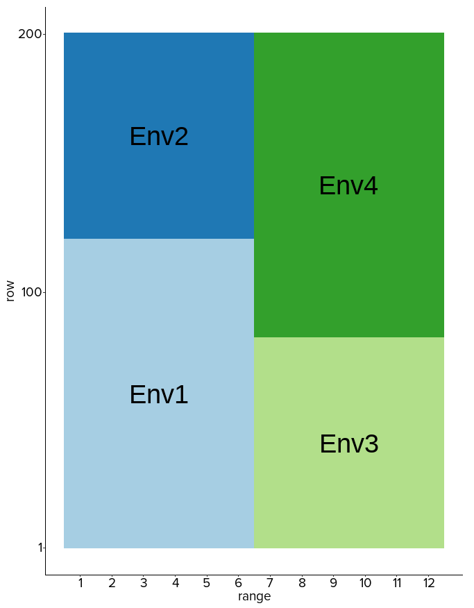
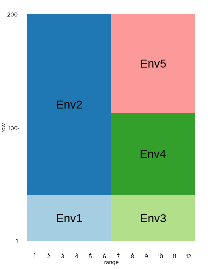
The PE approach

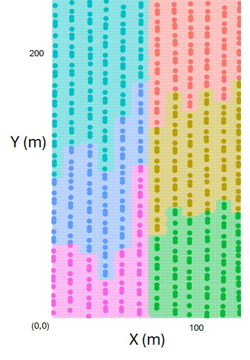
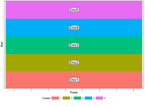
Pseudo-environments (PE) are created by grouping the grid points based on the spatial correlation structure (Stefanova et al. (2023)).
The PE approach is used to estimate the fixed effects.
The PE approach is for categorical variables.

The PE approach

The fifth element

BHM again to generate the synthetic data.

y_{i j k} = β_{0} + β_{{Env}_{i}} + β_{{Env}_{i} \times {variety}_{j}} + u_{{Env}_{i} \times {Rep}_{k}} + ϵ_{i j k}

$y_{ijk} = \beta_0 + \beta_{\text{Env}_i} + \beta_{\text{Env}_i \times \text{variety}_j} + u_{\text{Env}_i \times \text{Rep}_k} + \epsilon_{ijk}$ with:

u_{{Env}_{i} \times {Rep}_{k}} \sim N (0, σ_{{Env}_{i} \times {Rep}_{k}}^{2})

$u_{\text{Env}_i \times \text{Rep}_k} \sim \N(0, \sigma^2_{\text{Env}_i \times \text{Rep}_k})$ and:

ϵ_{i} \sim N (0, Σ_{i})

$\bm{\epsilon}_{i} \sim \N(0,\Sigma_i)$

The fifth element

Evaluation

The Mean Squared Error (MSE) for the fixed effects is calculated as:

{MSE}_{fixed} = \frac{1}{n} \sum_{i = 1}^{n} ({\hat{β}}_{i} - β_{i})^{2}

$\text{MSE}_{\text{fixed}} = \frac{1}{n} \sum_{i=1}^{n} (\hat{\beta}_i - \beta_i)^2$ where

{\hat{β}}_{i}

$\hat{\beta}_i$ are the estimated fixed effects and

β_{i}

$\beta_i$ are the true fixed effects.

The MSE for the random effects is calculated as:

{MSE}_{random} = \frac{1}{m} \sum_{j = 1}^{m} ({\hat{u}}_{j} - u_{j})^{2}

$\text{MSE}_{\text{random}} = \frac{1}{m} \sum_{j=1}^{m} (\hat{u}_j - u_j)^2$ where

{\hat{u}}_{j}

$\hat{u}_j$ are the estimated random effects and

u_{j}

$u_j$ are the true random effects.

Preliminary results

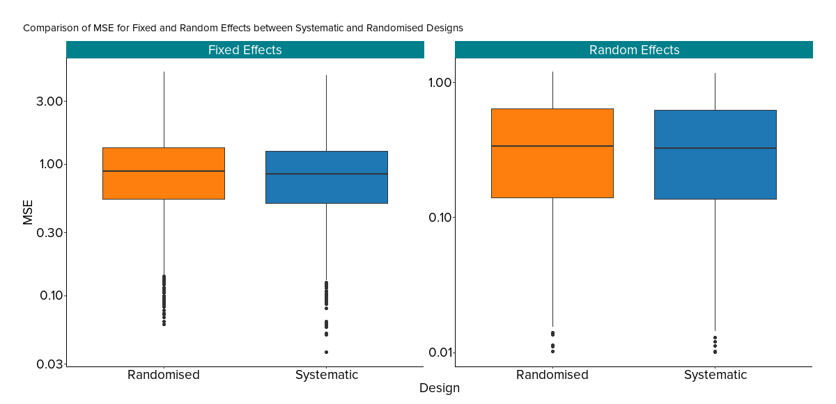
Preliminary results

MSE for fixed effects and random effects across different designs over 2000 iterations.

Type	Design	Mean	Median	Min	Max	Q1	Q3
Fixed Effects	Randomised	0.998	0.879	0.0605	5.02	0.542	1.33
Fixed Effects	Systematic	0.952	0.835	0.0369	4.76	0.503	1.26
Random Effects	Randomised	0.402	0.335	0.0102	1.19	0.140	0.637
Random Effects	Systematic	0.397	0.327	0.0100	1.17	0.138	0.626

Results

The puzzle is incomplete without the fifth piece.
The puzzle is still incomplete with the fifth piece.

Puzzles

Conclusion

A systematic design is superior to a randomised design for OFE when

spatial variation presents
quadratic response is assumed

Additionally,

the statement still holds for categorical variables
PE-approach shows it’s robustness in estimating fixed effects

Limitations

The proposed Bayesian approach is computationally intensive
The choice of parameters in the model can affect the results
For LMM PE approach, more variables can be incorporated

References

Cao, Zhanglong, Jordan Brown, Mark Gibberd, Julia Easton, and Suman Rakshit. 2024. “Optimal Design for on-Farm Strip Trials—Systematic or Randomised?” Field Crops Research 318: 109594.

Cao, Zhanglong, Katia Stefanova, Mark Gibberd, and Suman Rakshit. 2022. “Bayesian Inference of Spatially Correlated Random Parameters for on-Farm Experiment.” Field Crops Research 281: 108477.

Fotheringham, A Stewart, Chris Brunsdon, and Martin Charlton. 2003. Geographically Weighted Regression: The Analysis of Spatially Varying Relationships. John Wiley & Sons.

Gelman, Andrew, Aki Vehtari, Daniel Simpson, Charles C Margossian, Bob Carpenter, Yuling Yao, Lauren Kennedy, Jonah Gabry, Paul-Christian Bürkner, and Martin Modrák. 2020. “Bayesian Workflow.” arXiv Preprint arXiv:2011.01808.

Piepho, Hans-Peter, Christel Richter, Joachim Spilke, Karin Hartung, and Arndt Kunick. 2011. “Statistical Aspects of on-Farm Experimentation.” Crop & Pasture Science 62: 721–35. https://doi.org/10.1071/cp11175.

Rakshit, Suman, Adrian Baddeley, Katia Stefanova, Karyn Reeves, Kefei Chen, Zhanglong Cao, Fiona Evans, and Mark Gibberd. 2020. “Novel Approach to the Analysis of Spatially-Varying Treatment Effects in on-Farm Experiments.” Field Crops Research 255 (October 2019): 107783. https://doi.org/gg2vv7.

Stefanova, Katia T, Jordan Brown, Andrew Grose, Zhanglong Cao, Kefei Chen, Mark Gibberd, and Suman Rakshit. 2023. “Statistical Analysis of Comparative Experiments Based on Large Strip on-Farm Trials.” Field Crops Research 297: 108945.

Thank you.