Design and Spatial Analysis of On-Farm Strip Trials

From Principles to Simulation Evaluations

Zhanglong Cao, Julia Easton, Suman Rakshit, Barbara Kachigunda, Mark Gibberd

CCDM & EECMS, Curtin University

02/12/2025

Fundamental attributes of an experiment

• Replication

• Blocks

• Randomisation

(https://www.livingfarm.com.au)

What is on-farm experimentation?

Traditional research limitations

Small-plot trials: Limited relevance to commercial-scale farming

Controlled conditions: Don’t reflect real-world variability

Long translation time: Years between research and practice

Geographic specificity: Results may not transfer across regions

Farmer engagement: Limited involvement in research design

The OFE solution

Commercial-scale validation: Testing at realistic field sizes

Real-world conditions: Incorporating natural variability and farmer practices

Rapid innovation cycles: Faster feedback and adaptation

Local relevance: Site-specific recommendations

Farmer-scientist collaboration: Co-creation of knowledge

Illustration of OFE trial designs

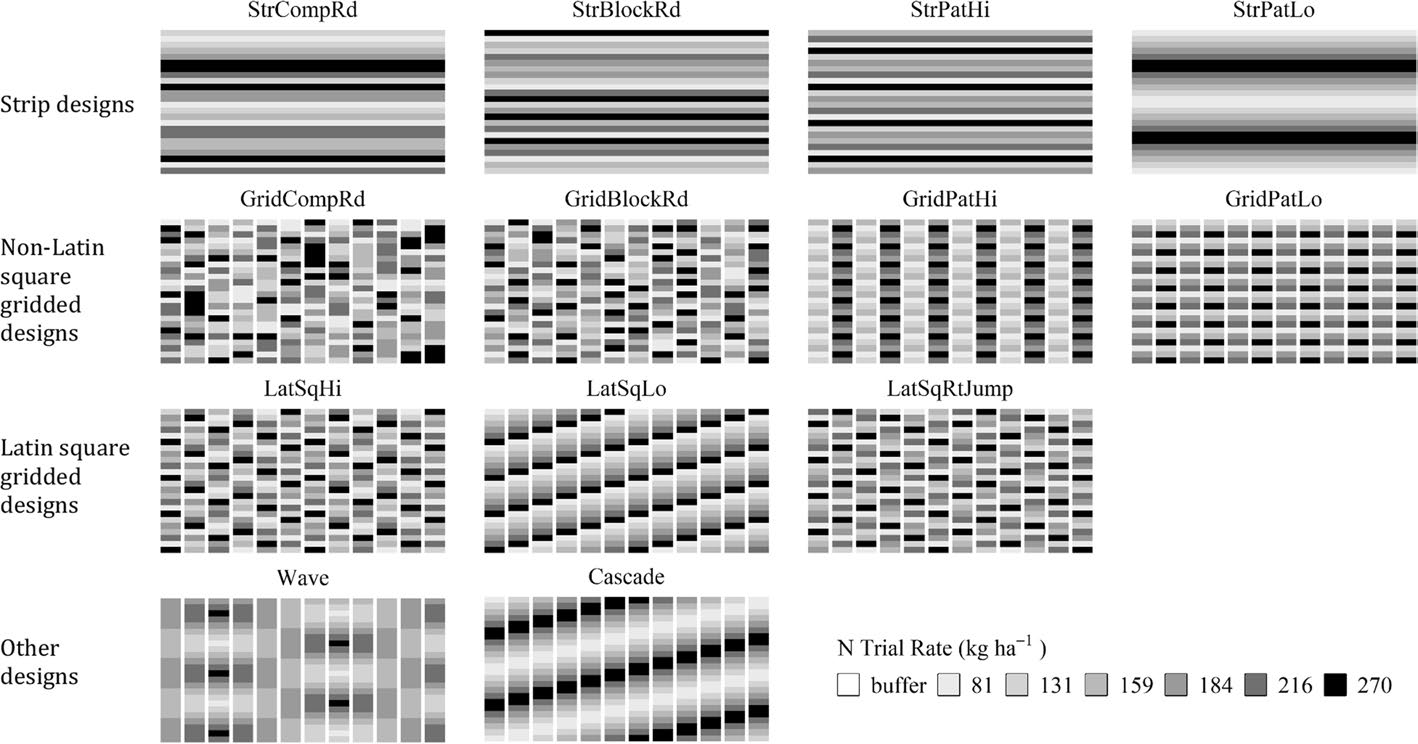
Illustration of some OFE trial designs, including strip-based, grid-based, Latin square, and gradient layouts. These designs support different analytical goals, such as treatment comparison, spatial modelling, and rate-response analysis (Li, Mieno, and Bullock (2023))

Why our focus is on strip trials?

Strip trial advantages for OFE

• Commercial compatibility: Matches farming operation scale
• Machinery integration: Works with standard farm equipment
• Cost efficiency: Lower setup and management costs
• Farmer adoption: Easy to implement and understand
• Practical relevance: Direct application to farm operations
• Precision agriculture: Compatible with variable-rate technology
• Technology integration: Works with GPS and yield monitors

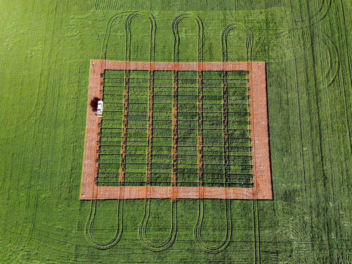
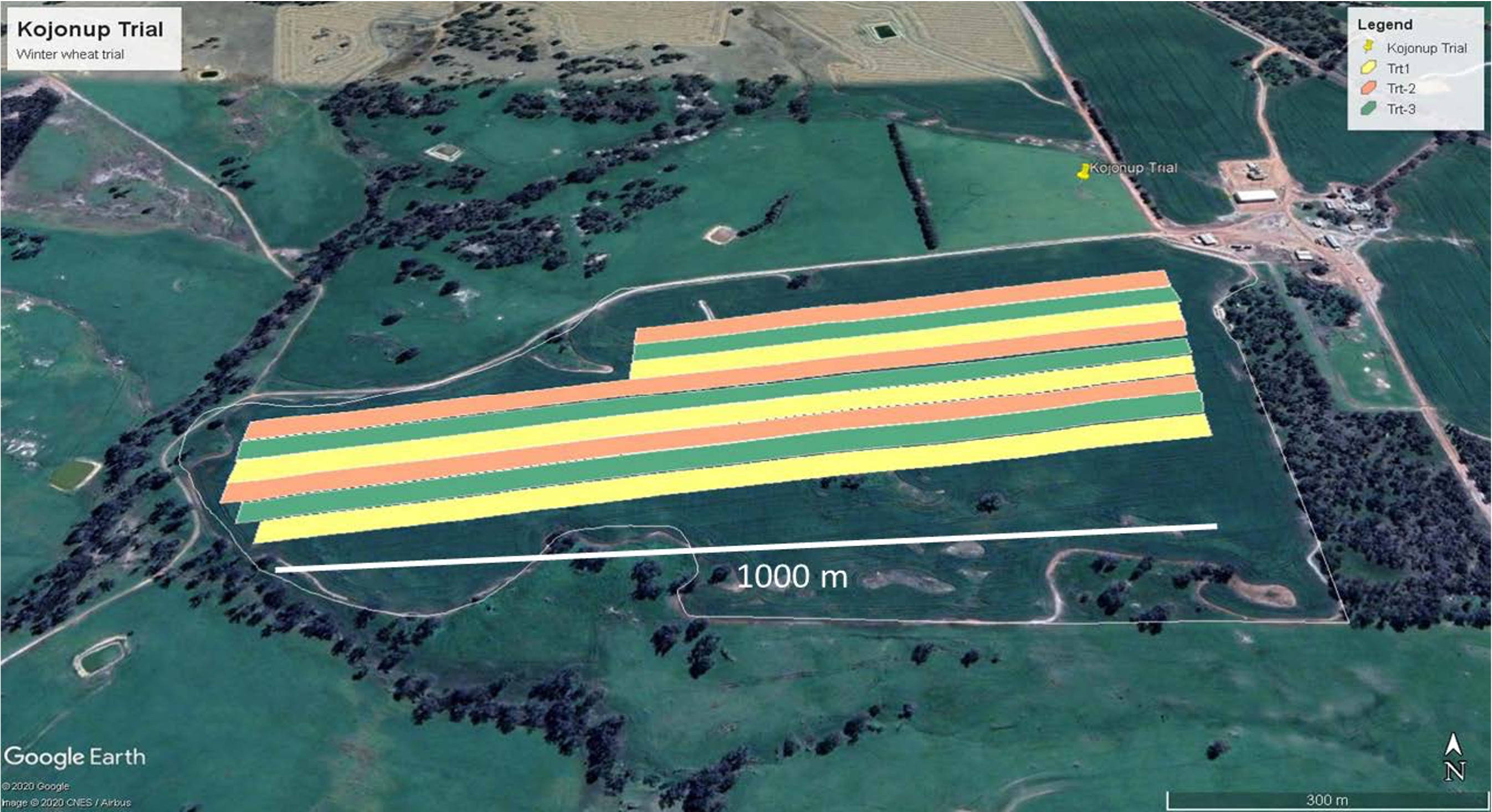
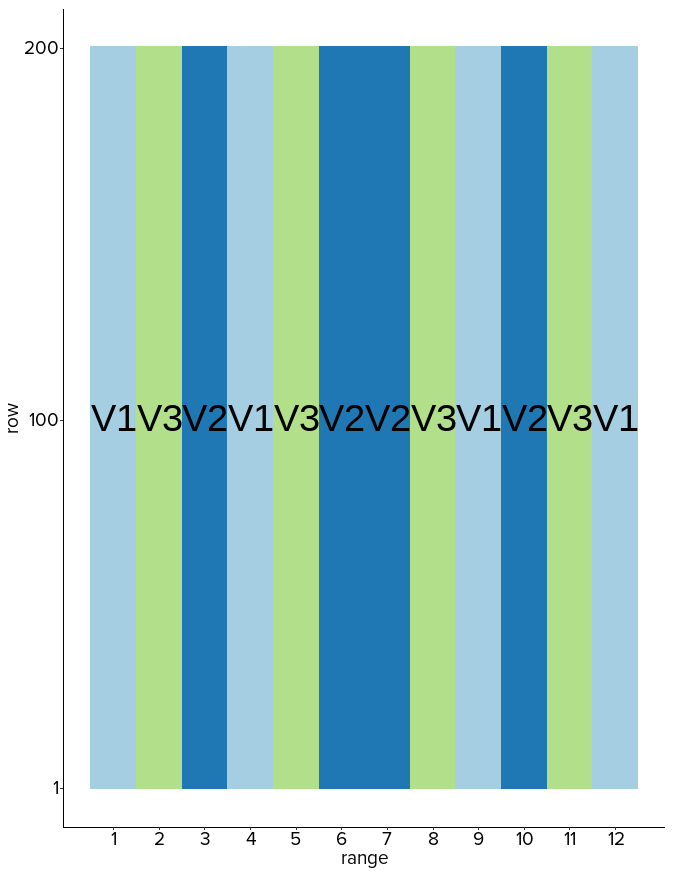
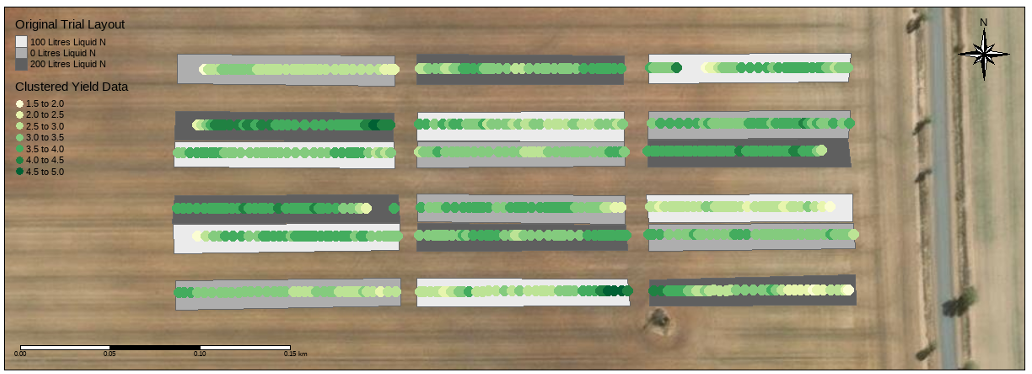
A typical long strip trial

Strip dimensions:

• Width: 10-30m (machinery width dependent)

• Length: 200m-1km (field size dependent)

• Area: 0.2-1.5 ha per strip

• Number: 2-6 treatments typical

A strip trial

Do these principles still hold for OFE

Traditional paradigm

• ✓ Replication

• ✓ Blocks

• ✓ Randomisation

Clear, controlled, artificial

OFE reality

• ? Replication (fewer reps)

• ? Blocks (natural variation)

• ? Randomisation (farmer constraints)

Practical, realistic, messy

Challenge: How to achieve statistical validity under OFE constraints?

Do these principles still hold for OFE

a randomised layout

a systematical layout

Previous studies on OFE design

For continuous responses, Prior research (Cao et al. 2022, 2024; Rakshit et al. 2020; Piepho et al. 2011; Pringle, Cook, and McBratney 2004) conclusively showed systematic designs outperform randomised designs for spatial analysis of continuous variables

Research focus

This study explores statistical strategies for the design and analysis of on-farm experiments (OFE), building on established foundations (Piepho et al. 2011; Pringle, Cook, and McBratney 2004) while advancing methodological innovation.

Do these design principles extend to categorical variables common in modern OFE?

Linear mixed model for OFE

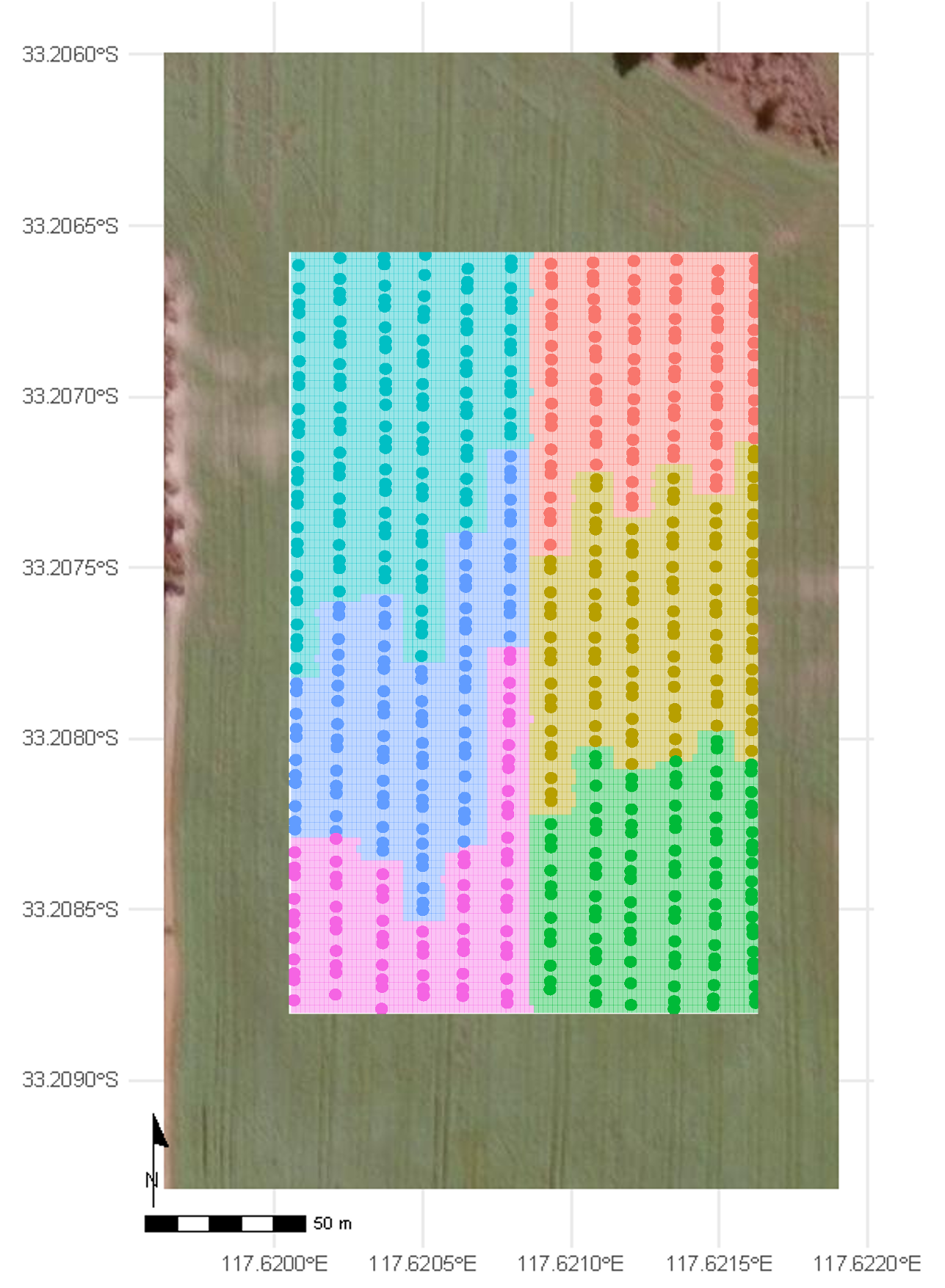
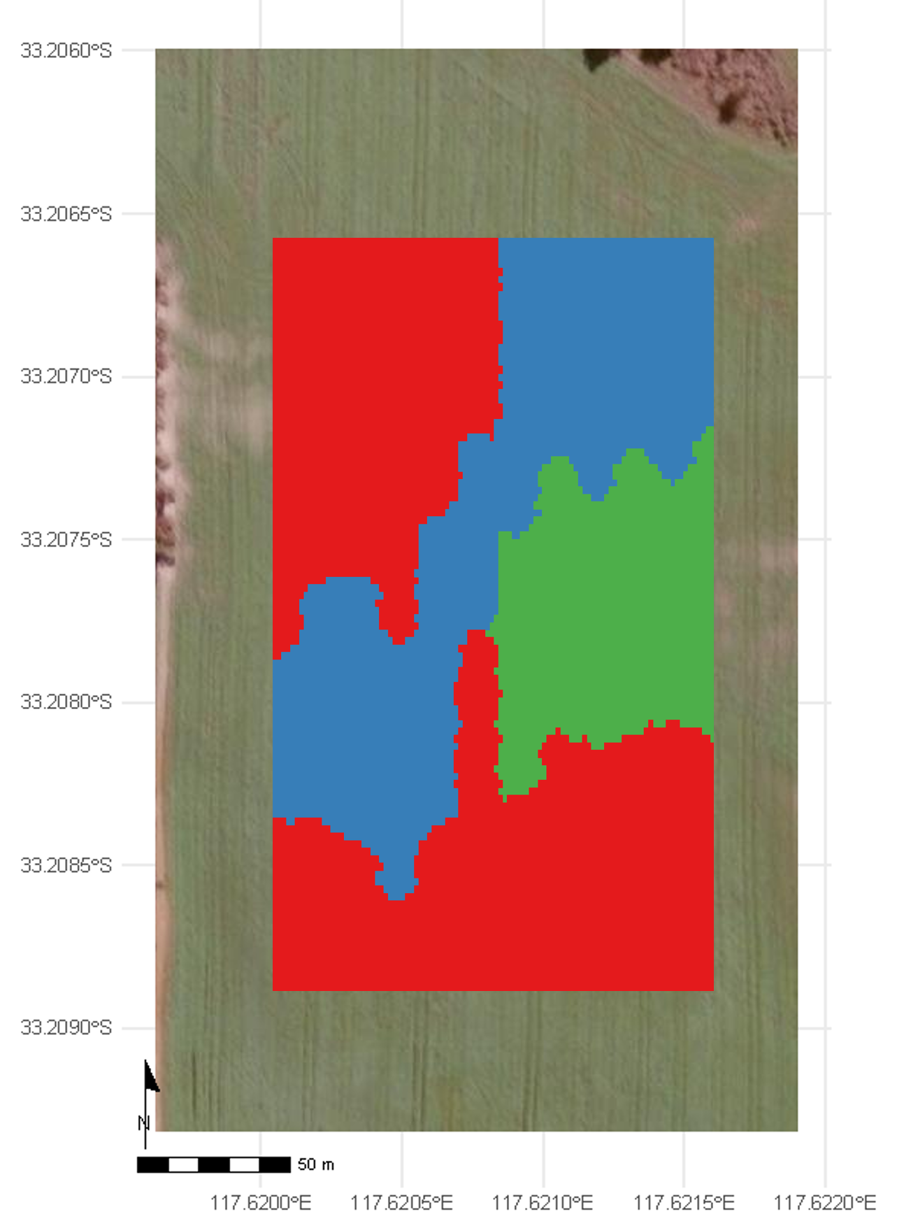
Core concept: Linear Mixed Models treat large strip OFEs similar to Multi-Environment Trials (MET), where pseudo-environments (PE) represent different zones within the field (Stefanova et al. (2023)).

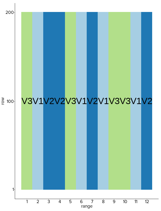
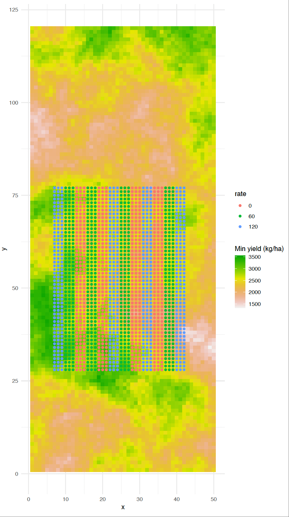
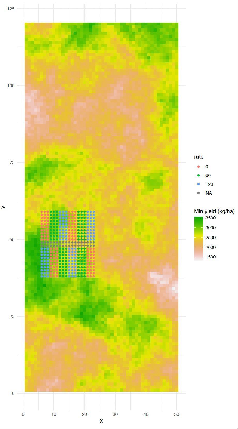
Linear mixed model for OFE

Suppose the entire field is partitioned into \(p\) PEs, and the \(j\)th PE consists of \(n_j\) grid points, such that the total number of grid points in the experiment is \(n=\sum_{j=1}^p n_j\). Let \({y}_j\) be the \(n_{j} \times 1\) vector of observed responses corresponding to the \(j\)th PE. The LMM for the combined vector of data \({Y} = \lbrack{y}^\top_{1}, \ldots, {y}^\top_{p}\rbrack^{\top}\) across all PEs is given by \[\begin{equation}\label{eq:modelmatrix} {Y} = {X}{\tau} + {Z}{u} + {e}, \end{equation}\] where \({\tau}\) and \({u}\) are \(t\times 1\) and \(b \times 1\) vectors of fixed and random effects, respectively. The matrices \({X}\) and \({Z}\) are \(n\times t\) and \(n\times b\) design matrices corresponding to the fixed and random effects, respectively. The \(n\times 1\) vector \({e}\) provides the combined residual effects from all PEs.

Typically, the random effect \({u} = \lbrack {u}^{\top}_{1}, \ldots, {u}^{\top}_{q}\rbrack^{\top}\) is composed of several model terms, with the corresponding design matrix \({Z}\) partitioned as \(\lbrack {Z}_1, \ldots,{Z}_q \rbrack\).

Linear mixed model for OFE

Why PEs matter:

• Fields are not uniform - different zones behave differently

• One-size-fits-all recommendations often fail

• Zone-specific management improves overall performance

Practical implementation:

• Clustering approach using elevation, soil, or other covariates

• Systematic partitioning when covariates unavailable

• 3-6 zones typically optimal for most fields

• Statistical modeling within each zone

Linear mixed model for OFE

The map shows the best-performing treatment for each pseudo-environment (PE) as estimated by the LMM (Stefanova et al. (2023)).

Interpretation

• The LMM identifies which treatment yields the highest predicted response in each PE.
• This enables zone-specific recommendations, supporting precision management.
• Spatial patterns reflect underlying field heterogeneity and treatment × environment interactions.

Simulation study - LMM

We simulate baseline yield using unconditional Gaussian geo-statistical simulation based on a first-order stationary random field model (Evans et al. (2020)). \[ z(s) = \mu + \varepsilon(s) \] where \(z(s)\) is the simulated yield at location \(s = (x, y)\), fertiliser trials are simulated using different designs and is added to the baseline yield: \[ y(s) = z(s) + \beta \times N(s) \]

Simulation study - LMM

Primary research question

How do trial length, number of replications, model structure (spatial vs non-spatial), data granularity (averaged vs full), and layout (strip vs stacked) affect the accuracy and statistical power of treatment effect estimation in OFE?

• Trial length: Short (100 m) to long (1100 m) strips/trials
• Replications: 2 to 12
• Model types: Non-spatial (M11, M21), spatial (M12, M22, M23)
• Data granularity: Averaged data (mean yield per strip/zone) vs full data (all yield points)
• Design layouts: Strip and stacked replicated trials

Stacked replicated design

This design is especially useful when:

• Field length is limited, but replication is still required.

• High-resolution spatial data is available, allowing for detailed modelling.

Stacked Layout

Simulation study - LMM

Result for strip trials

Boxplots of relative absolute difference (RAD) across different trial lengths, models, and designs of coefficients of strip trials. Each panel represents a combination of trial length and model (M11–M22), with RAD values compared between randomised and systematic strip designs. Lower RAD values indicate more accurate treatment effect estimation. Randomised designs and models incorporating spatial terms (M12,M22) show improved performance.

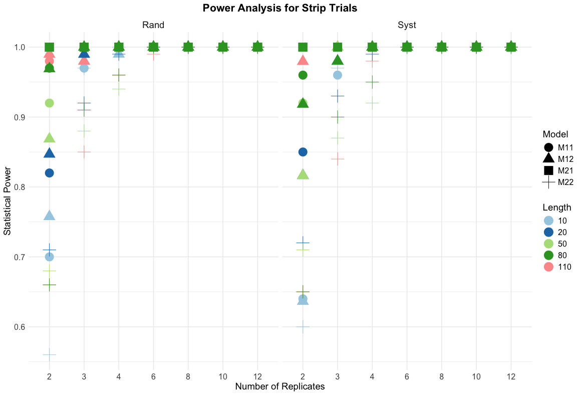
Statistical powers of strip trials

Key findings for strip trials

Critical Design Thresholds

Minimum 3 replications required for 95%+ power in most scenarios

Strip length matters: Longer strips (\(\ge\) 500m) show consistent power improvement

Spatial models (M12, M22) enhance power by 5-15% over non-spatial models

Full data analysis consistently outperforms averaged data approaches

Design-specific performance

Randomised designs: Superior power for hypothesis testing (0.85-1.0 typical)

Systematic designs: Adequate power (0.70-0.95) with operational advantages

Length effect: 1100m strips achieve 98%+ power with 2 reps vs 70% for 100m strips

Model selection: Spatial correlation models critical for realistic field conditions

Result for stacked trials

Boxplots of relative absolute difference (RAD) for stacked replicate trials across different trial lengths and models. Each panel represents a combination of trial length and model (M11–M23), with RAD values compared between randomised and systematic designs. While randomised designs generally show slightly lower RAD values, the differences are less pronounced than in strip trials.

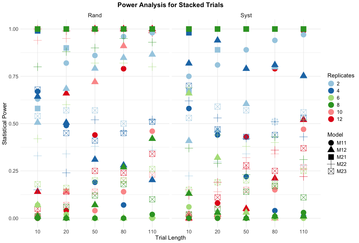
Statistical powers of stacked trials

Key findings for stacked trials

Critical performance patterns:

• M21 (Full non-spatial): Consistently achieves 100% power across all scenarios

• M23 models: Generally poor performance (0.1-0.7 power) - avoid in practice

• Length sensitivity: Dramatic improvement from 10m (0.0-0.7) to 110m (0.25-1.0) trials

• Replication effects: Optimal performance at 10-12 reps, diminishing returns beyond 6 reps

Model selection insights:

• Averaged data models: Highly variable power (0.0-1.0) - unreliable for inference

• Full data analysis: More consistent and higher power overall

• Spatial vs non-spatial: Non-spatial models (M21) surprisingly outperform spatial models (M22, M23)

• Design comparison: Randomised slightly better than systematic, but differences minimal

Practical recommendations: For stacked trials, prioritize M21 models with full data analysis and ensure adequate trial length (\(\ge\) 50m) for reliable statistical inference.

Data collection

Yield monitor technology

Combine harvesters: Real-time yield measurement

GPS integration: Precise location recording

Data logging: Continuous data capture at 1-second intervals

Quality sensors: Moisture, protein, oil content measurement

Auxiliary spatial data

NDVI or multispectral imagery for vegetation indices

Soil electrical conductivity from dual EM surveys

Gamma radiometric data for soil texture

Digital elevation models (DEM) for topographic variation

Weather station data for environmental context

Soil moisture sensors for irrigation management

Method selection framework

Objective-driven design: Select design strategy based on research goals and intended analytical approach

LMM for: categorical treatments & zone-based analysis

Categorical comparisons: Varieties, formulations, products

Hypothesis testing: Statistical significance of treatment effects

Zone-specific management: Different areas of the field

Treatment × environment interactions: How treatments perform across zones

GWR for continuous treatments & spatial optimisation

Continuous treatments: Varying nitrogen rates, seeding rates

Spatial optimisation: Site-specific management

Variable-rate applications: Precision agriculture implementation

Local response mapping: Understanding spatial variability

National standard and research impact

Adoption as standard operating procedures

• These guidelines form the basis for standard operating procedures (SOPs) for OFE trial design and analysis in Australia.
• Widely adopted by research organisations, grower groups, and industry partners as the benchmark for OFE methodology.
• Referenced in national projects and used to train researchers and practitioners.
• Collaborators and partners have implemented these standards in their OFE projects.
• Ensures consistency, scientific rigor, and practical relevance across diverse environments and research teams.

National standard and research impact

Our research outputs are not just academic—they set the national standard for on-farm experimentation, guiding the next generation of agricultural innovation in Australia. – Zhanglong Cao

Acknowledgements

This research and presentation were made possible through the support and collaboration of:

• GRDC (Grains Research & Development Corporation)

• Australian Grower Groups (Liebe Group, Facey Group, Grower Group Alliance, Consult Ag, Delta Agribusiness, Riverine Plains, Sygenta, Coterva, NSW DPI, DPIRD, DPI QLD and more)

Special thanks to all collaborating farmers, research staff, and postgraduate students for their contributions to on-farm experimentation and data collection.

Acknowledgements

Special thanks to EECMS, CBADA, C4AP & CCDM Curtin University

Thank you!

Reference

Cao, Zhanglong, Jordan Brown, Mark Gibberd, Julia Easton, and Suman Rakshit. 2024. “Optimal Design for on-Farm Strip Trials—Systematic or Randomised?” Field Crops Research 318: 109594.

Cao, Zhanglong, Katia Stefanova, Mark Gibberd, and Suman Rakshit. 2022. “Bayesian Inference of Spatially Correlated Random Parameters for on-Farm Experiment.” Field Crops Research 281: 108477.

Evans, Fiona H., Angela Recalde Salas, Suman Rakshit, Craig A. Scanlan, and Simon E. Cook. 2020. “Assessment of the Use of Geographically Weighted Regression for Analysis of Large On-Farm Experiments and Implications for Practical Application.” Agronomy 10 (11): 1720. https://doi.org/10.3390/agronomy10111720.

Li, Xiaofei, Taro Mieno, and David S Bullock. 2023. “The Economic Performances of Different Trial Designs in on-Farm Precision Experimentation: A Monte Carlo Evaluation.” Precision Agriculture 24 (6): 2500–2521. https://doi.org/10.1007/s11119-023-10050-8.

Piepho, Hans-Peter, Christel Richter, Joachim Spilke, Karin Hartung, Arndt Kunick, and Heinrich Thöle. 2011. “Statistical Aspects of on-Farm Experimentation.” Crop and Pasture Science 62 (9): 721–35.

Pringle, MJ, SE Cook, and AB McBratney. 2004. “Field-Scale Experiments for Site-Specific Crop Management. Part i: Design Considerations.” Precision Agriculture 5 (6): 617–24. https://doi.org/10.1007/s11119-004-6344-y.

Rakshit, Suman, Adrian Baddeley, Katia Stefanova, Karyn Reeves, Kefei Chen, Zhanglong Cao, Fiona Evans, and Mark Gibberd. 2020. “Novel Approach to the Analysis of Spatially-Varying Treatment Effects in on-Farm Experiments.” Field Crops Research 255 (September): 107783. https://doi.org/10.1016/j.fcr.2020.107783.

Stefanova, Katia T., Jordan Brown, Andrew Grose, Zhanglong Cao, Kefei Chen, Mark Gibberd, and Suman Rakshit. 2023. “Statistical Analysis of Comparative Experiments Based on Large Strip on-Farm Trials.” Field Crops Research 297 (June): 108945. https://doi.org/10.1016/j.fcr.2023.108945.