All Posts
Browse all articles and research updates
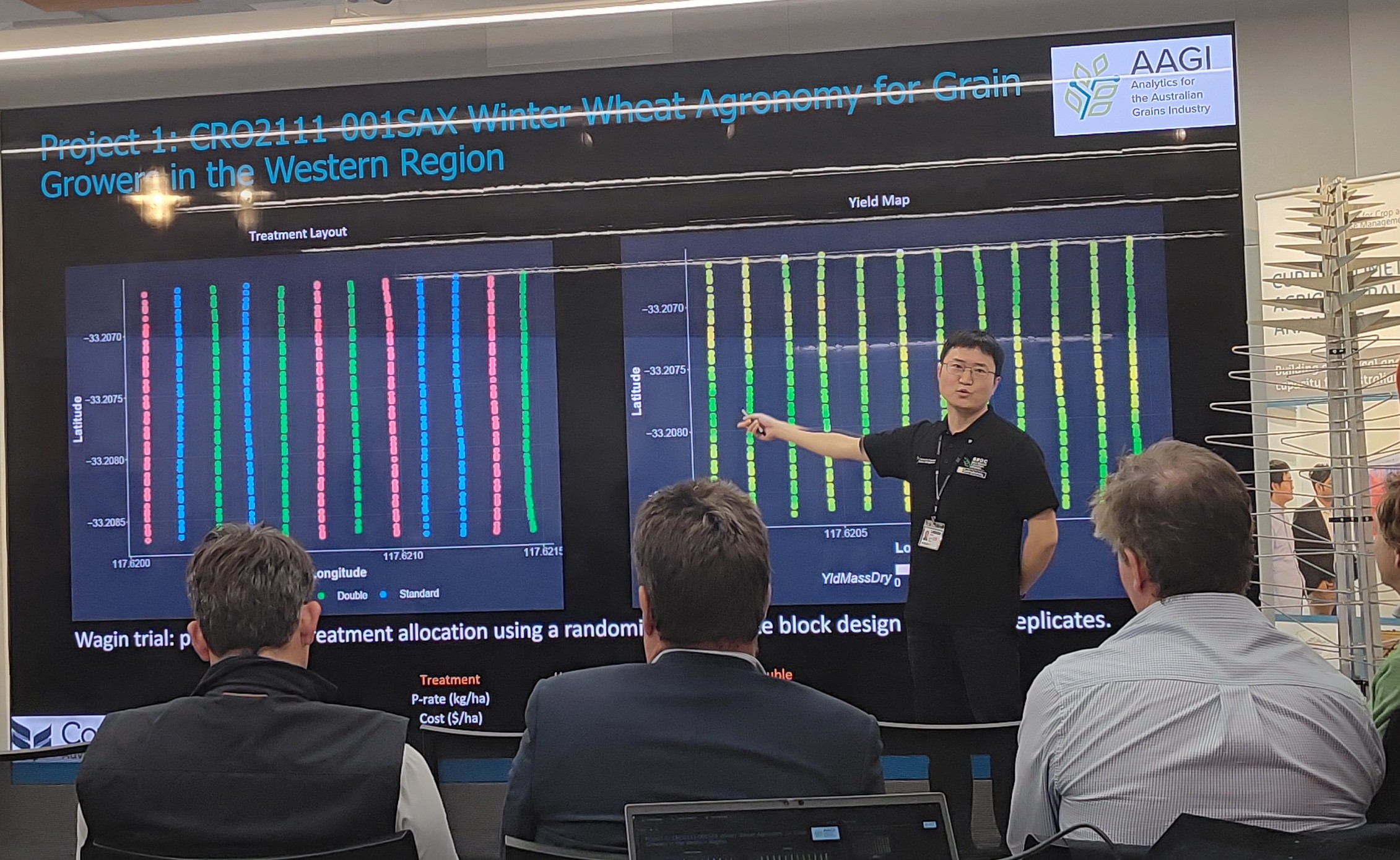
Open Day Web App Demo: Turning Data into Interactive Stories
Open Day Web App Demo
Mortgage Mate — Support & FAQ
Mortgage Mate — Support & FAQ 🏡
Mortgage Mate: A Data-Driven Home Loan Simulator for Australian Buyers
Mortgage Mate 🏡
MenuMate is Live on the App Store! 🎉
After months of design, development, and late nights, I’m incredibly excited to announce that MenuMate (AI点菜助手) has officially been approved by Apple and is now live on the App Store! 🍽️🚀
MenuMate: AI-Powered Menu Assistant - updated
MenuMate 🍽️
PromptlySocial: My New iOS App for Social Media Posts
Hey everyone! I just launched a new iOS app called PromptlySocial that I think you’ll find useful if you’re struggling with what to post on social media.
ASC Perth: Design and Spatial Analysis of On-Farm Strip Trials – From Principles to Simulation Evaluations
I presented at the Australian Statistical Conference (ASC) in Perth (December 2025), sharing a comprehensive study on statistical strategies for the design and analysis of on-farm strip trials, bridging foundational experimental design principles with modern spatial modelling and simulation evaluations.
IBS Canberra: Bayesian Ordinal Regression for Crop Development and Disease Assessment
I presented at the International Biometric Society (IBS) meeting in Canberra (November 2025), sharing recent developments in Bayesian ordinal regression methods for analysing crop development and disease severity data from field trials.
ANU Seminar: Design and Spatial Analysis of On-Farm Strip Trials
Yesterday, I had the pleasure of presenting at the Australian National University (ANU) seminar series. The presentation focused on statistical strategies for the design and analysis of on-farm experiments, from fundamental principles to simulation evaluations.
🎓 New Beginnings at EECMS: Lecturer in Statistics
This week marks an exciting new chapter in my academic career — I’ve joined the School of Electrical Engineering, Computing and Mathematical Sciences (EECMS) at Curtin University as a Lecturer.
OZWeatherApp: AI-Powered Australian Weather & Climate Insights
🌦️ OZWeatherApp
Launching Stats Journey – A Statistics Learning Platform
Proving the Superiority of Systematic Designs in On-Farm Trials
Presentation at AASC 2024
This is the presentation that I gave on 4th September at AASC 2024 Rottnest Island.
Case Studies in Advanced Analysis of Large Strip On-farm Experiments
Abstract: On-farm experiments (OFE) are gaining attention among farmers and agronomists for testing various research questions on real farms. The Analytics for the Australian Grains Industry (AAGI) has developed several techniques for analysing OFE data. Geographically Weighted Regression (GWR) and the multi-environment trial (MET) technique, which partitions paddocks into pseudo-environments (PEs), have proven effective. Additionally, we have explored the potential of the Generalised Additive Model (GAM) for handling temporal and spatial variability, given its flexibility in accommodating non-linear variables. In this presentation, we will demonstrate case studies using these techniques to analyse OFE data and compare the outcomes of different approaches.
Presentation at Pawsey Centre
This is the 5-minute presentation that I gave to GRDC western panel and growers at Pawsey Centre..
Analytics Innovations in On-farm Experiments
A Deep Spatio-temporal Gaussian Process for Yield Prediction in West Australia
In the realm of precision farming, the application of Machine Learning (ML) and Deep Learning (DL) algorithms has proven to be invaluable for analyzing and modeling agricultural data that varies across both space and time. While most research has heavily leaned toward utilizing remote sensing data, particularly in image recognition, the advancements in deep learning methodologies for regression problems have been comparatively slow.
Regression techniques are crucial for large-scale agricultural trials, especially when the goal is to identify optimal management practices for specific locations within a field. To enhance predictive accuracy, it’s essential to incorporate various factors—topographical, environmental, and ground conditions—into the modeling process.
To address this gap, our recent work introduces an innovative framework that leverages spatio-temporal estimation and prediction of agricultural data through deep learning and Gaussian processes. By integrating a deep Gaussian Process component, we explicitly model the spatio-temporal structure of the data, while utilizing standard deep learning techniques to account for other influential factors.
We applied our framework to two real-world datasets, demonstrating its effectiveness and accuracy in yield prediction. This approach not only enhances our understanding of agricultural dynamics but also paves the way for more informed decision-making in precision farming.
Stay tuned for further insights as we delve deeper into the applications and implications of this research!
An Introduction to RShiny
It’s a workshop provided to introduce participants to RShiny, a powerful web application framework for R. During this workshop, attendees will learn how to create interactive web applications that can visualize data and facilitate user input.
Workshop Overview
The workshop will cover the following key topics:
- Introduction to R and Shiny: Understanding the basics of R and how it integrates with Shiny.
- Creating a Simple Shiny App: Step-by-step guidance on building your first Shiny application.
- UI and Server Components: Exploring the user interface (UI) and server functions that make up a Shiny app.
- Reactive Programming: Learning how to make applications responsive to user input.
- Data Visualization: Using libraries like ggplot2 to create dynamic plots within Shiny apps.
- Deployment: Overview of how to deploy Shiny apps to shinyapps.io or a local server.
Target Audience
This workshop is aimed at R users who want to enhance their data analysis skills by creating interactive web applications. No prior experience with Shiny is required, but a basic understanding of R programming is recommended.
Objectives
By the end of the workshop, participants will be able to:
- Develop a basic Shiny application.
- Understand the key components of Shiny apps.
- Implement interactive features to enhance user experience.
- Deploy their applications for public access.
Resources
Participants will be provided with:
- Workshop materials, including example code and data.
- Access to recorded sessions for future reference.
- Support for any follow-up questions after the workshop.
A Bayesian Workflow for Spatially Correlated Random Effects in On-farm Experiment
Check out the embedded Quarto HTML file below:
Optimal design for on-farm strip trials --- systematic or randomised?
There is no doubt on the importance of randomisation in agricultural experiments by agronomists and biometricians. Even when agronomists extend the experimentation from small trials to large on-farm trials, randomised designs predominate over systematic designs at most times.
However, the situation maybe changed depending on the objective of the on-farm experiments (OFE). If the goal of OFE is obtaining a smooth map showing the optimal level of a controllable input across a grid made by rows and columns covering the whole field, a systematic design should be preferred over a randomised design in terms of robustness and reliability.
With the novel geographically weighted regression (GWR) for OFE and simulation studies, we conclude that, for large OFE strip trials, the difference between randomised designs and systematic designs are not significant if the assumption is linear response and the spatial variation is not taken into account. However, systematic designs are superior to randomised designs if the assumption of the response is quadratic.
Confounded treatment and blocking
Confounded Treatment and Blocking Structure
Encounted a problem that the treatment is confounded with the blocking structure. In this situation, it is not possible to assess the interaction of the treatment and genotypes.
Example
Here is an example of the trial:
set.seed(1234)
Rep <- rep(as.vector(replicate(2,sample(c("Rep1","Rep2","Rep3"),3))),each=5)
Gens <- paste0("Gen",1:5)
Geno <- as.vector(replicate(6, sample(Gens,5)))
TOS <- rep(c("TOS1","TOS2"),each=15)
Rows <- rep(1:5,6)
Cols <- rep(1:6,each=5)
dat <- data.frame(Rows,Cols,Rep,Geno,TOS)
ggplot(dat) + geom_tile(aes(Cols,Rows,fill=Rep))
ggplot(dat) + geom_tile(aes(Cols,Rows,fill=TOS))
ggplot(dat) + geom_tile(aes(Cols,Rows,fill=Geno))
dat$y <- 3+rnorm(length(Rep))
names(dat)## [1] "Rows" "Cols" "Rep" "Geno" "TOS" "y"nms <- c("Rows","Cols","Rep","Geno","TOS")
dat[nms] <- lapply(dat[nms], factor)The researchers would like to assess the effects of different Time of Sowing, Genotypes and their interactions on a set of traits.
Model 1
With the trial, the interaction is not possibly being assessed because the treatment is confounded with the blocking structure.
mod1 <- asreml(y ~ TOS*Geno,
random = ~ TOS:Rep,
data = dat)## Online License checked out Thu Mar 4 16:57:37 2021
## Model fitted using the gamma parameterization.
## ASReml 4.1.0 Thu Mar 4 16:57:37 2021
## LogLik Sigma2 DF wall cpu
## 1 -12.0709 0.654877 20 16:57:37 0.0
## 2 -12.0484 0.644739 20 16:57:37 0.0
## 3 -12.0259 0.624656 20 16:57:37 0.0
## 4 -12.0256 0.622321 20 16:57:37 0.0plot(mod1)
wald(mod1,denDF = "default",ssType = "conditional")## Model fitted using the gamma parameterization.
## ASReml 4.1.0 Thu Mar 4 16:57:37 2021
## LogLik Sigma2 DF wall cpu
## 1 -12.0256 0.622286 20 16:57:37 0.0
## 2 -12.0256 0.622286 20 16:57:37 0.0
## 3 -12.0256 0.622286 20 16:57:37 0.0## $Wald
## [0;34m
## Wald tests for fixed effects.[0m
## [0;34mResponse: y[0m
##
## Df denDF F.inc F.con Margin Pr
## (Intercept) 1 4 131.600 131.600 0.00033
## TOS 1 4 0.003 0.003 A 0.95740
## Geno 4 16 0.394 0.394 A 0.80986
## TOS:Geno 4 16 0.619 0.619 B 0.65513
##
## $stratumVariances
## df Variance TOS:Rep units!R
## TOS:Rep 4 1.1778601 5 1
## units!R 16 0.6222861 0 1Model 2
The two TOS blocks were treated as two different environments. As such, a MET analysis techniques were used assuming heterogeneous variance for both TOS.
mod2 <- asreml(y ~ TOS + Geno,
random = ~ at(TOS):Rep,
data = dat)## Model fitted using the gamma parameterization.
## ASReml 4.1.0 Thu Mar 4 16:57:37 2021
## LogLik Sigma2 DF wall cpu
## 1 -12.3657 0.609972 24 16:57:37 0.0
## 2 -12.3039 0.599510 24 16:57:37 0.0
## 3 -12.2332 0.579837 24 16:57:37 0.0
## 4 -12.2288 0.575302 24 16:57:37 0.0## Warning in asreml(y ~ TOS + Geno, random = ~at(TOS):Rep, data = dat): Some
## components changed by more than 1% on the last iteration.plot(mod2)
wald(mod2,denDF = "default",ssType = "conditional")## Model fitted using the gamma parameterization.
## ASReml 4.1.0 Thu Mar 4 16:57:38 2021
## LogLik Sigma2 DF wall cpu
## 1 -12.2287 0.574921 24 16:57:38 0.0
## 2 -12.2287 0.574920 24 16:57:38 0.0
## 3 -12.2287 0.574918 24 16:57:38 0.0## $Wald
## [0;34m
## Wald tests for fixed effects.[0m
## [0;34mResponse: y[0m
##
## Df denDF F.inc F.con Margin Pr
## (Intercept) 1 3.8 138.100 138.100 0.00039
## TOS 1 3.8 0.003 0.003 A 0.95753
## Geno 4 20.0 0.427 0.427 A 0.78766
##
## $stratumVariances
## df Variance at(TOS, TOS1):Rep at(TOS, TOS2):Rep units!R
## at(TOS, TOS1):Rep 2 1.4385847 5 -2.297635e-17 1
## at(TOS, TOS2):Rep 2 0.9171355 0 5.000000e+00 1
## units!R 20 0.5749179 0 0.000000e+00 1Hans-Peter has a paper discussing this issue and an example shows that there is complete confounding of area and treatment effects. So the model 1 in our case is not valid.
References
- Hans-Peter Piepho, Mian Faisal Nazir, M. Kausar Nawaz Shah (2016). Design and analysis of a trial to select for stress tolerance. COMMUNICATIONS IN BIOMETRY AND CROP SCIENCE. VOL. 11, NO. 1, 2016, PP. 1–9
A note on estimating Lmm With Reml And Bayesian Approaches
A note on estimating LMM with REML and Bayesian approaches
I encountered that REML and Bayesian approahes treat the random term \(u\) of a linear mixed model differently.
Suppose we have a linear mixed model \[\begin{equation} y=X\beta + Zu+e, \end{equation}\] with \(E[u]=0\), \(E[e]=0\) and \[\begin{equation} Var \begin{bmatrix} u \\ e \end{bmatrix} = \begin{bmatrix} G & 0 \\ 0 & R \end{bmatrix}. \end{equation}\]
REML
REML has the assumption that \[\begin{align} E[y] &= X\beta \\ Var[y] &= ZGZ^\top+R. \end{align}\] Then it calculates the BLUP in the following way that \[\begin{align} X^\top R^{-1}X\hat{\beta} + X^\top R^{-1}Z\hat{u} &= X^\top R^{-1} y \\ Z^\top R^{-1} X\hat{\beta} + (Z^\top R^{-1} Z +G^{-1})\hat{u} &= Z^\top R^{-1} y \end{align}\] which, further with \(V = ZGZ^\top + R\), are \[\begin{align} \hat{\beta} &= (X^\top V^{-1}X)^{-1} X^\top V^{-1}y\\ \hat{u} &= (Z^\top R^{-1} Z+G^{-1})^{-1}Z^\top R^{-1}(I - X(X^\top V^{-1}X)^{-1}X^\top V^{-1})y \\ &= GZ^\top V^{-1}(I - X(X^\top V^{-1}X)^{-1}X^\top V^{-1})y \end{align}\]
Bayesian
Alternatively, Bayesian analysis uses \[\begin{align} E[y] &= X\beta + Zu \\ Var[y] &= R. \end{align}\] It is different from maximum likelihood approaches, Bayesian approaches treat \(u\) as model parameters in the same manner as \(\beta\) rather than assuming it is part of the error term. In this way, the uncertainty in its estimates can be naturally evaluated .
Then the Bayesian inference will be \[\begin{equation} p(\theta\mid y) \propto p(y\mid\theta)\pi(\theta), \end{equation}\] which is also called the marginal posterior distribution. The distribution of \(p(\theta\mid y)\) is the ``Bayesian inference’’ of the parameter because all information about \(\theta\) is contained in the distribution. Then, by taking natural logarithm on the posterior, for multivariate Gaussian distribution, we will have \[\begin{equation} L(\theta) \propto -\frac{1}{2} (y-X\beta-Zu)^\top R^{-1}(y-X\beta-Zu) -\frac{1}{2}\ln\det R + \ln \pi(\theta), \end{equation}\]
Presentation at SAGI Symposium 2020
This is the joint presentation by me and Suman at SAGI Symposium 2020.
Part 1 is given by Suman about OFE and GWR approach. The detail is at publication.
Title: On-farm Strip Trials: going beyond small plot experiments
Abstract: Accommodating spatial variation is common in analysing field trials, and has become a challenge in large on-farm experiments. Simple linear mixed models and Gaussian distribution are incapable of dealing with complex data sets and results in misspecification. This paper describes a Bayesian framework to analyse the model with spatially correlated random parameters for large on-farm experiments. With advanced model diagnostic tools, we found that the model with Gaussian assumption is misspecified. Therefore, we use Student distribution with which the model is augmented. The open-source R-code that implements our proposed method for analysing on-farm data is provided for further use. We also discuss the difference of the Bayesian approach and GWR, and compare the results from these two approaches.
Good PP check and R square but large Pareto k values
Recently, I encountered a problem with using PSIS and Pareto k for model diagnostics and selection. Some models have good posterior predictive checking performance but a few terrible Pareto k values. And sometimes, a model with more high k values might be misspecified.
A discussion is at Stan forum.
Single Site Ofe
Single Site OFE
Data visualization
The data set is lasrosas.corn from the R-package agridat. The yield monitor data for a corn field (quintals/ha) was conducted by incorporating six nitrogen rate treatments in three replicated blocks comprising 18 strips across the field in Argentina in 2001. The raw data is converted to 93 rows \(\times\) 18 cols grid.
summary(gridded_df_ordered)## x y yield nitro
## Min. :-5137122 Min. :-6258764 Min. : 12.66 Min. : 0.0
## 1st Qu.:-5136910 1st Qu.:-6258727 1st Qu.: 50.51 1st Qu.: 39.0
## Median :-5136707 Median :-6258689 Median : 84.66 Median : 63.0
## Mean :-5136705 Mean :-6258689 Mean : 75.32 Mean : 64.9
## 3rd Qu.:-5136504 3rd Qu.:-6258650 3rd Qu.: 99.52 3rd Qu.: 99.8
## Max. :-5136293 Max. :-6258613 Max. :117.90 Max. :124.6
##
## topo bv rep nf StripNo RowId
## E :350 Min. : 91.74 R1:558 N0:279 Strip: 1: 93 Min. : 1
## HT:414 1st Qu.:168.10 R2:558 N1:279 Strip: 2: 93 1st Qu.:24
## LO:424 Median :173.63 R3:558 N2:279 Strip: 3: 93 Median :47
## W :486 Mean :174.67 N3:279 Strip: 4: 93 Mean :47
## 3rd Qu.:180.26 N4:279 Strip: 5: 93 3rd Qu.:70
## Max. :213.82 N5:279 Strip: 6: 93 Max. :93
## (Other) :1116
## row col cnitro nitro.sq cnitro.sq
## 1 : 18 1 : 93 Min. :-64.9 Min. : 0 Min. : 110.2
## 2 : 18 2 : 93 1st Qu.:-25.9 1st Qu.: 1521 1st Qu.: 204.5
## 3 : 18 3 : 93 Median : -1.9 Median : 4123 Median : 944.4
## 4 : 18 4 : 93 Mean : 0.0 Mean : 5875 Mean :1663.3
## 5 : 18 5 : 93 3rd Qu.: 34.9 3rd Qu.: 9960 3rd Qu.:3564.1
## 6 : 18 6 : 93 Max. : 59.7 Max. :15525 Max. :4212.0
## (Other):1566 (Other):1116
## gridobject gridId
## 1 : 6 1 : 1
## 2 : 6 2 : 1
## 3 : 6 3 : 1
## 4 : 6 4 : 1
## 5 : 6 5 : 1
## 6 : 6 6 : 1
## (Other):1638 (Other):1668ggplot(gridded_df_ordered) + geom_point(aes(row,col,colour=rep),size=2) + theme_bw()
ggplot(gridded_df_ordered) + geom_point(aes(row,col,colour=nf),size=2) + theme_bw()
ggplot(gridded_df_ordered) + geom_point(aes(row,col,colour=yield),size=2) + theme_bw()
ggplot(gridded_df_ordered) + geom_point(aes(row,col,colour=topo),size=2) + theme_bw()
ggplot(gridded_df_ordered, aes(x= yield,y=topo,fill=topo)) +
geom_density_ridges()## Picking joint bandwidth of 3.01
countplot <- gridded_df_ordered
countplot$x1<- as.numeric(countplot$row)
countplot$y1<- as.numeric(countplot$col)
coordinates(countplot) <- c("x1", "y1")
spplot(countplot, "yield")
countplot.ppp <- as(countplot["yield"], "ppp")
countplot.ppp.smooth <- Smooth(countplot.ppp)
plot(countplot.ppp.smooth, col=matlab.like2, ribsep=0.01,
ribside="bottom", main="")
contour(countplot.ppp.smooth,"marks.nitro", add=TRUE, lwd=1,
vfont=c("sans serif", "bold italic"), labcex=0.9)
Models
df <- read.csv("SinglesiteModel.csv")
kable(df)%>%kable_styling(bootstrap_options = c("striped", "hover"))| X | Fixed | Random | Residual | Log.likelihood | AIC | BIC |
|---|---|---|---|---|---|---|
| model 0 | 1 | rep+nf | — | -6266.143 | 12538.290 | 12554.550 |
| model 1 | 1 | rep+nf | id(row):id(col) | -6266.143 | 12538.290 | 12554.550 |
| model 2 | 1+lin(row)+lin(col) | rep+nf | ar1(row):ar1(col) | -3913.398 | 7836.796 | 7863.902 |
| model 3 | 1+lin(row) | rep+nf+spl(row) | ar1(row):ar1(col) | -3607.354 | 7226.708 | 7259.238 |
| model 4 | 1+lin(row) | rep+nf+spl(row)+outl | ar1(row):ar1(col) | -3441.974 | 6897.948 | 6935.900 |
| model 5 | 1+lin(row)+nf | rep+spl(row)+outl | ar1(row):ar1(col) | -3434.315 | 6880.630 | 6913.143 |
| model 6 | 1+lin(row)+nf+lin(row):nf | rep+spl(row)+outl | ar1(row):ar1(col) | -3450.218 | 6912.436 | 6944.931 |
| model 7 | 1+lin(row)+nf | rep+spl(row)+outl+nf:spl(row) | ar1(row):ar1(col) | -3430.177 | 6874.353 | 6912.284 |
| model 8 | 1+cnitro+cnitro.sq | rep | ar1(row):ar1(col) | -3922.920 | 7853.840 | 7875.525 |
| model 9 | 1+lin(row)+cnitro+cnitro.sq | rep+spl(row) | ar1(row):ar1(col) | -3611.849 | 7233.698 | 7260.801 |
| model 10 | 1+lin(row)+cnitro+cnitro.sq | rep+spl(row)+outl | ar1(row):ar1(col) | -3446.323 | 6904.646 | 6937.170 |
| model 11 | 1+lin(row)+cnitro+cnitro.sq | rep+spl(row)+outl+cnitro:spl(row)+cnitro.sq:spl(row) | ar1(row):ar1(col) | -3438.807 | 6893.614 | 6936.979 |
Fit treatment as random
#initial model
mod0 <- asreml(yield ~ 1,
random= ~ rep+nf,
data=gridded_df_ordered, maxiter=20)## Model fitted using the gamma parameterization.
## ASReml 4.1.0 Tue Jul 21 09:37:00 2020
## LogLik Sigma2 DF wall cpu
## 1 -6273.834 652.480 1673 09:37:00 0.0 (2 restrained)
## 2 -6267.399 654.012 1673 09:37:00 0.0 (1 restrained)
## 3 -6266.281 654.396 1673 09:37:00 0.0 (1 restrained)
## 4 -6266.152 654.576 1673 09:37:00 0.0 (1 restrained)
## 5 -6266.144 654.571 1673 09:37:00 0.0 (1 restrained)
## 6 -6266.143 654.571 1673 09:37:00 0.0asrmod(mod0)## $loglik
## [1] -6266.143
##
## $AIC
## [1] 12538.29
## attr(,"parameters")
## [1] 3
##
## $BIC
## [1] 12554.55
## attr(,"parameters")
## [1] 3plot(mod0)
mod1 <- asreml(yield ~ 1,
random= ~ rep+nf,
residual= ~ id(row):id(col),
data=gridded_df_ordered)## Model fitted using the gamma parameterization.
## ASReml 4.1.0 Tue Jul 21 09:37:02 2020
## LogLik Sigma2 DF wall cpu
## 1 -6273.834 652.480 1673 09:37:02 0.0 (2 restrained)
## 2 -6267.399 654.012 1673 09:37:02 0.0 (1 restrained)
## 3 -6266.281 654.396 1673 09:37:02 0.0 (1 restrained)
## 4 -6266.152 654.576 1673 09:37:02 0.0 (1 restrained)
## 5 -6266.144 654.571 1673 09:37:02 0.0 (1 restrained)
## 6 -6266.143 654.571 1673 09:37:02 0.0asrmod(mod1)## $loglik
## [1] -6266.143
##
## $AIC
## [1] 12538.29
## attr(,"parameters")
## [1] 3
##
## $BIC
## [1] 12554.55
## attr(,"parameters")
## [1] 3summary(mod1,param="gamma")$varcomp## gamma component std.error z.ratio bound %ch
## rep 1.011929e-07 6.623795e-05 2.293633e-06 28.8790582 B 0
## nf 4.658895e-03 3.049578e+00 3.413517e+00 0.8933832 P 0
## row:col!R 1.000000e+00 6.545712e+02 2.266595e+01 28.8790582 P 0#check the significance of the fixed effects
wald(mod1)## [0;34mWald tests for fixed effects.[0m
## [0;34mResponse: yield[0m
## [0;34mTerms added sequentially; adjusted for those above.[0m
##
## Df Sum of Sq Wald statistic Pr(Chisq)
## (Intercept) 1 4129124 6308.1 < 2.2e-16 ***
## residual (MS) 655
## ---
## Signif. codes: 0 '***' 0.001 '**' 0.01 '*' 0.05 '.' 0.1 ' ' 1#run the diagnostics
plot(varioGram(mod1))
plot(mod1)
#fit the linear column and linear row effects model
mod2 <- asreml(yield ~ 1+lin(row)+lin(col),
random= ~ rep+nf,
residual= ~ar1(row):ar1(col),
data=gridded_df_ordered,maxiter=30)## Model fitted using the gamma parameterization.
## ASReml 4.1.0 Tue Jul 21 09:37:04 2020
## LogLik Sigma2 DF wall cpu
## 1 -5673.261 323.517 1671 09:37:04 0.0 (3 restrained)
## 2 -4615.786 126.868 1671 09:37:04 0.0 (2 restrained)
## 3 -3997.362 134.557 1671 09:37:04 0.0 (1 restrained)
## 4 -3963.913 161.589 1671 09:37:04 0.0 (1 restrained)
## 5 -3919.907 300.788 1671 09:37:04 0.0 (2 restrained)
## 6 -3913.614 345.522 1671 09:37:04 0.0 (1 restrained)
## 7 -3913.406 337.173 1671 09:37:04 0.0 (1 restrained)
## 8 -3913.398 341.281 1671 09:37:04 0.0
## 9 -3913.398 340.286 1671 09:37:04 0.0#diagnostics
asrmod(mod2)## $loglik
## [1] -3913.398
##
## $AIC
## [1] 7836.796
## attr(,"parameters")
## [1] 5
##
## $BIC
## [1] 7863.902
## attr(,"parameters")
## [1] 5# -3913.398
summary(mod2)$varcomp## component std.error z.ratio bound %ch
## rep 3.443454e-05 5.571003e-06 6.181031 B 0
## nf 8.883445e-05 1.437211e-05 6.181031 B 0
## row:col!R 3.402861e+02 5.505330e+01 6.181031 P 0
## row:col!row!cor 9.374610e-01 1.068600e-02 87.727923 U 0
## row:col!col!cor 2.639157e-01 2.502896e-02 10.544416 U 0wald(mod2)## [0;34mWald tests for fixed effects.[0m
## [0;34mResponse: yield[0m
## [0;34mTerms added sequentially; adjusted for those above.[0m
##
## Df Sum of Sq Wald statistic Pr(Chisq)
## (Intercept) 1 277682 816.03 < 2.2e-16 ***
## lin(row) 1 2981 8.76 0.003077 **
## lin(col) 1 37 0.11 0.743124
## residual (MS) 340
## ---
## Signif. codes: 0 '***' 0.001 '**' 0.01 '*' 0.05 '.' 0.1 ' ' 1plot(varioGram(mod2))
plot(mod2)
# lin(col) is not significant, add spline row
mod3 <- asreml(yield~ 1+lin(row),
random= ~rep+nf+spl(row),
residual= ~ar1(row):ar1(col),
data=gridded_df_ordered,maxit=30)## Model fitted using the gamma parameterization.
## ASReml 4.1.0 Tue Jul 21 09:37:06 2020
## Spline: design points closer than 0.0092 have been merged.
## LogLik Sigma2 DF wall cpu
## 1 -3736.861 30.5672 1672 09:37:06 0.1 (1 restrained)
## 2 -3671.982 29.3929 1672 09:37:06 0.1
## 3 -3624.633 29.7522 1672 09:37:07 0.1
## 4 -3609.884 31.0471 1672 09:37:07 0.1
## 5 -3607.429 32.0617 1672 09:37:07 0.1
## 6 -3607.356 32.2887 1672 09:37:07 0.1
## 7 -3607.354 32.3363 1672 09:37:07 0.1asrmod(mod3)#$loglik## $loglik
## [1] -3607.354
##
## $AIC
## [1] 7226.708
## attr(,"parameters")
## [1] 6
##
## $BIC
## [1] 7259.238
## attr(,"parameters")
## [1] 6# -3607.354
summary(mod3)$varcomp## component std.error z.ratio bound %ch
## rep 0.1837729 0.36505126 0.5034168 P 0.1
## nf 5.1187964 3.41221249 1.5001400 P 0.0
## spl(row) 9.8298245 2.96299498 3.3175299 P 0.0
## row:col!R 32.3362912 1.36943864 23.6128075 P 0.0
## row:col!row!cor 0.4415356 0.02081960 21.2076837 U 0.1
## row:col!col!cor 0.1486154 0.02568646 5.7857458 U 0.0wald(mod3)## [0;34mWald tests for fixed effects.[0m
## [0;34mResponse: yield[0m
## [0;34mTerms added sequentially; adjusted for those above.[0m
##
## Df Sum of Sq Wald statistic Pr(Chisq)
## (Intercept) 1 188245 5821.5 < 2.2e-16 ***
## lin(row) 1 91584 2832.2 < 2.2e-16 ***
## residual (MS) 32
## ---
## Signif. codes: 0 '***' 0.001 '**' 0.01 '*' 0.05 '.' 0.1 ' ' 1plot(varioGram(mod3))
plot(mod3)
###############################################
# identify outliers
mod3.aom <- update(mod3,aom=T)## Model fitted using the gamma parameterization.
## ASReml 4.1.0 Tue Jul 21 09:37:09 2020
## Spline: design points closer than 0.0092 have been merged.
## LogLik Sigma2 DF wall cpu
## 1 -3607.354 32.3452 1672 09:37:09 0.1
## 2 -3607.354 32.3458 1672 09:37:09 0.1
## 3 -3607.354 32.3470 1672 09:37:09 0.1# gridded_df_ordered$aom <- residuals(mod3.aom)
gridded_df_ordered$aom <- mod3.aom$aom$R[,2]
ggplot(gridded_df_ordered) + geom_histogram(aes(aom),binwidth=1) +
ggtitle("Histogram of Standardised Residuals")+theme_bw()
# ggplot(gridded_df_ordered) + geom_boxplot(aes(topo,aom)) + theme_bw()
# standardised residual plots of model 3
mod3.1 <- mod3
mod3.1$residuals<- mod3.aom$aom$R[,2]
plot(mod3.1)
temp <- gridded_df_ordered
order(gridded_df_ordered$aom)[1:10]## [1] 74 1490 1116 1239 1369 1670 943 1473 1531 57wh <- which(abs(gridded_df_ordered$aom)>5)
resID <- c(74)
gridded_df_ordered[resID,]## x y yield nitro topo bv rep nf StripNo RowId row col
## 510 -5137046 -6258749 19.41 75.4 W 177.46 R1 N3 Strip: 2 5 5 2
## cnitro nitro.sq cnitro.sq gridobject gridId aom
## 510 10.5 5685.16 110.25 5 74 -17.228gridded_df_ordered$outl <- 0
gridded_df_ordered$outl[resID] <- 1
gridded_df_ordered$outl <- as.factor(gridded_df_ordered$outl)
# removing extreme outliers
gridded_df_ordered$yield[74] <- NA
mod3.2 <- asreml(yield~ 1+lin(row),
random= ~rep+nf+spl(row),
residual= ~ar1(row):ar1(col),
data=gridded_df_ordered,maxit=30)## Model fitted using the gamma parameterization.
## ASReml 4.1.0 Tue Jul 21 09:37:11 2020
## Spline: design points closer than 0.0092 have been merged.
## LogLik Sigma2 DF wall cpu
## 1 -3628.468 26.9187 1671 09:37:11 0.1 (1 restrained)
## 2 -3528.873 25.1916 1671 09:37:11 0.1
## 3 -3460.926 25.5634 1671 09:37:11 0.1
## 4 -3440.607 27.1242 1671 09:37:11 0.1
## 5 -3437.212 28.4171 1671 09:37:11 0.1
## 6 -3437.106 28.7254 1671 09:37:11 0.1
## 7 -3437.102 28.7894 1671 09:37:11 0.1
## 8 -3437.102 28.8016 1671 09:37:11 0.1asrmod(mod3.2)#$loglik## $loglik
## [1] -3437.102
##
## $AIC
## [1] 6886.204
## attr(,"parameters")
## [1] 6
##
## $BIC
## [1] 6918.731
## attr(,"parameters")
## [1] 6summary(mod3.2)$varcomp## component std.error z.ratio bound %ch
## rep 0.1996678 0.39200006 0.5093566 P 0
## nf 5.2028157 3.47688797 1.4964002 P 0
## spl(row) 9.3337692 2.71290752 3.4405040 P 0
## row:col!R 28.8015509 1.29788494 22.1911435 P 0
## row:col!row!cor 0.5118910 0.02010364 25.4626049 U 0
## row:col!col!cor 0.1479415 0.02593579 5.7041445 U 0wald(mod3.2)## [0;34mWald tests for fixed effects.[0m
## [0;34mResponse: yield[0m
## [0;34mTerms added sequentially; adjusted for those above.[0m
##
## Df Sum of Sq Wald statistic Pr(Chisq)
## (Intercept) 1 163993 5693.9 < 2.2e-16 ***
## lin(row) 1 76586 2659.1 < 2.2e-16 ***
## residual (MS) 29
## ---
## Signif. codes: 0 '***' 0.001 '**' 0.01 '*' 0.05 '.' 0.1 ' ' 1plot(varioGram(mod3.2))
plot(mod3.2)
mod3.2.aom <- update(mod3.2,aom=T)## Model fitted using the gamma parameterization.
## ASReml 4.1.0 Tue Jul 21 09:37:13 2020
## Spline: design points closer than 0.0092 have been merged.
## LogLik Sigma2 DF wall cpu
## 1 -3437.102 28.8039 1671 09:37:13 0.1
## 2 -3437.102 28.8041 1671 09:37:14 0.1
## 3 -3437.102 28.8044 1671 09:37:14 0.1gridded_df_ordered$aom2 <- mod3.2.aom$aom$R[,2]
ggplot(gridded_df_ordered) + geom_histogram(aes(aom2),binwidth=1) +
ggtitle("Histogram of Standardised Residuals")+theme_bw()
order(gridded_df_ordered$aom2)[1:10]## [1] 1490 1116 1239 1369 1670 943 1473 719 1131 1531resID <- c(74,which(abs(gridded_df_ordered$aom2)>2))
gridded_df_ordered[resID,]## x y yield nitro topo bv rep nf StripNo RowId row col
## 510 -5137046 -6258749 NA 75.4 W 177.46 R1 N3 Strip: 2 5 5 2
## 110 -5137080 -6258749 87.73 75.4 W 166.49 R1 N3 Strip: 2 1 1 2
## 1101 -5137122 -6258613 86.66 39.0 W 142.55 R3 N1 Strip: 18 1 1 18
## 270 -5137105 -6258647 100.52 75.4 W 139.78 R3 N3 Strip: 14 2 2 14
## 2101 -5137113 -6258613 102.16 39.0 W 131.17 R3 N1 Strip: 18 2 2 18
## 412 -5137063 -6258741 91.04 99.8 W 174.33 R1 N4 Strip: 3 4 4 3
## 460 -5137088 -6258656 110.90 124.6 W 96.39 R3 N5 Strip: 13 4 4 13
## 570 -5137080 -6258647 80.05 75.4 W 171.65 R3 N3 Strip: 14 5 5 14
## 580 -5137079 -6258639 85.22 99.8 W 172.75 R3 N4 Strip: 15 5 5 15
## 5101 -5137088 -6258614 99.69 39.0 W 171.22 R3 N1 Strip: 18 5 5 18
## 610 -5137038 -6258749 108.03 75.4 W 173.70 R1 N3 Strip: 2 6 6 2
## 650 -5137071 -6258639 108.45 99.8 W 174.05 R3 N4 Strip: 15 6 6 15
## 812 -5137029 -6258741 100.54 99.8 W 177.22 R1 N4 Strip: 3 8 8 3
## 9 -5137013 -6258758 100.44 124.6 W 179.49 R1 N5 Strip: 1 9 9 1
## 920 -5137038 -6258690 76.03 99.8 W 176.80 R2 N4 Strip: 9 9 9 9
## 1112 -5137021 -6258690 78.20 99.8 W 175.24 R2 N4 Strip: 9 11 11 9
## 121 -5136987 -6258750 81.90 75.4 W 183.94 R1 N3 Strip: 2 12 12 2
## 128 -5137004 -6258699 49.13 75.4 W 185.62 R2 N3 Strip: 8 12 12 8
## 13 -5136979 -6258758 82.70 124.6 W 180.27 R1 N5 Strip: 1 13 13 1
## 23 -5136894 -6258759 62.98 124.6 W 181.74 R1 N5 Strip: 1 23 23 1
## 259 -5136902 -6258683 36.08 0.0 W 177.30 R2 N0 Strip: 10 25 25 10
## 2615 -5136910 -6258632 36.09 0.0 W 181.43 R3 N0 Strip: 16 26 26 16
## 3315 -5136851 -6258632 31.38 0.0 HT 171.74 R3 N0 Strip: 16 33 33 16
## 3614 -5136817 -6258641 37.03 99.8 HT 188.19 R3 N4 Strip: 15 35 35 15
## 3917 -5136800 -6258616 52.90 39.0 HT 202.74 R3 N1 Strip: 18 38 38 18
## 4013 -5136783 -6258650 34.62 75.4 HT 198.83 R3 N3 Strip: 14 39 39 14
## 4117 -5136775 -6258650 43.70 75.4 HT 203.71 R3 N3 Strip: 14 40 40 14
## 4118 -5136775 -6258641 32.05 99.8 HT 204.97 R3 N4 Strip: 15 40 40 15
## 4120 -5136783 -6258624 31.79 50.6 HT 203.68 R3 N2 Strip: 17 40 40 17
## 4218 -5136775 -6258625 47.02 50.6 HT 202.14 R3 N2 Strip: 17 41 41 17
## 423 -5136742 -6258735 12.66 0.0 HT 193.16 R1 N0 Strip: 4 42 42 4
## 442 -5136725 -6258743 32.90 99.8 HT 187.79 R1 N4 Strip: 3 44 44 3
## 4516 -5136749 -6258625 50.57 50.6 HT 182.88 R3 N2 Strip: 17 44 44 17
## 4713 -5136732 -6258616 62.88 39.0 HT 179.37 R3 N1 Strip: 18 46 46 18
## 5218 -5136690 -6258625 68.11 50.6 HT 182.17 R3 N2 Strip: 17 50 50 17
## 5212 -5136673 -6258676 47.52 50.6 E 177.43 R2 N2 Strip: 11 51 51 11
## 531 -5136640 -6258753 75.83 75.4 E 177.89 R1 N3 Strip: 2 52 52 2
## 546 -5136648 -6258710 58.28 124.6 E 176.14 R2 N5 Strip: 7 53 53 7
## 547 -5136648 -6258702 74.35 75.4 E 175.50 R2 N3 Strip: 8 53 53 8
## 548 -5136657 -6258693 63.75 99.8 E 178.95 R2 N4 Strip: 9 53 53 9
## 556 -5136640 -6258710 87.78 124.6 E 177.27 R2 N5 Strip: 7 54 54 7
## 5415 -5136648 -6258634 69.74 0.0 E 173.77 R3 N0 Strip: 16 54 54 16
## 5614 -5136648 -6258642 65.65 99.8 E 177.05 R3 N4 Strip: 15 55 55 15
## 5717 -5136648 -6258617 81.37 39.0 E 173.73 R3 N1 Strip: 18 55 55 18
## 5817 -5136639 -6258617 101.34 39.0 E 174.48 R3 N1 Strip: 18 56 56 18
## 583 -5136606 -6258736 103.97 0.0 E 170.44 R1 N0 Strip: 4 57 57 4
## 5915 -5136605 -6258634 91.11 0.0 E 171.43 R3 N0 Strip: 16 59 59 16
## 6118 -5136605 -6258643 98.81 99.8 E 171.22 R3 N4 Strip: 15 60 60 15
## 6015 -5136597 -6258634 102.16 0.0 E 171.42 R3 N0 Strip: 16 60 60 16
## 635 -5136572 -6258719 105.73 39.0 E 176.47 R1 N1 Strip: 6 61 61 6
## 645 -5136564 -6258719 97.94 39.0 E 177.19 R1 N1 Strip: 6 62 62 6
## 6414 -5136580 -6258643 111.74 99.8 E 175.66 R3 N4 Strip: 15 62 62 15
## 6416 -5136588 -6258626 109.24 50.6 E 164.57 R3 N2 Strip: 17 62 62 17
## 6417 -5136588 -6258618 81.00 39.0 E 163.03 R3 N1 Strip: 18 62 62 18
## 655 -5136555 -6258719 106.84 39.0 E 169.45 R1 N1 Strip: 6 63 63 6
## 6514 -5136572 -6258643 95.77 99.8 E 167.74 R3 N4 Strip: 15 63 63 15
## 6516 -5136580 -6258626 92.21 50.6 E 168.51 R3 N2 Strip: 17 63 63 17
## 6811 -5136538 -6258669 110.54 39.0 E 161.69 R2 N1 Strip: 12 66 66 12
## 6916 -5136546 -6258626 96.32 50.6 E 167.79 R3 N2 Strip: 17 67 67 17
## 708 -5136521 -6258694 98.09 99.8 E 169.45 R2 N4 Strip: 9 68 68 9
## 7016 -5136538 -6258626 112.85 50.6 E 170.98 R3 N2 Strip: 17 68 68 17
## 7112 -5136513 -6258694 111.87 99.8 E 171.61 R2 N4 Strip: 9 69 69 9
## 7118 -5136521 -6258643 90.45 99.8 E 169.94 R3 N4 Strip: 15 69 69 15
## 7313 -5136504 -6258652 94.33 75.4 E 165.49 R3 N3 Strip: 14 71 71 14
## 734 -5136479 -6258728 93.06 50.6 LO 169.12 R1 N2 Strip: 5 72 72 5
## 7414 -5136495 -6258644 98.88 99.8 E 161.76 R3 N4 Strip: 15 72 72 15
## 744 -5136471 -6258729 108.01 50.6 LO 162.02 R1 N2 Strip: 5 73 73 5
## 7614 -5136478 -6258644 117.90 99.8 LO 162.17 R3 N4 Strip: 15 74 74 15
## 76 -5136446 -6258763 95.93 124.6 LO 169.89 R1 N5 Strip: 1 75 75 1
## 77 -5136437 -6258763 116.64 124.6 LO 159.75 R1 N5 Strip: 1 76 76 1
## 78 -5136429 -6258763 97.56 124.6 LO 163.36 R1 N5 Strip: 1 77 77 1
## 7914 -5136453 -6258644 112.94 99.8 LO 172.52 R3 N4 Strip: 15 77 77 15
## 8113 -5136428 -6258687 107.59 0.0 LO 169.97 R2 N0 Strip: 10 79 79 10
## 8118 -5136436 -6258644 87.43 99.8 LO 163.91 R3 N4 Strip: 15 79 79 15
## 813 -5136412 -6258746 112.83 99.8 LO 170.25 R1 N4 Strip: 3 80 80 3
## 8211 -5136420 -6258687 94.65 0.0 LO 165.06 R2 N0 Strip: 10 80 80 10
## 8417 -5136419 -6258619 107.22 39.0 LO 164.82 R3 N1 Strip: 18 81 81 18
## 83 -5136386 -6258763 110.56 124.6 LO 163.70 R1 N5 Strip: 1 82 82 1
## 8413 -5136411 -6258653 100.51 75.4 LO 153.08 R3 N3 Strip: 14 82 82 14
## 8414 -5136411 -6258644 92.60 99.8 LO 161.18 R3 N4 Strip: 15 82 82 15
## 8513 -5136402 -6258653 69.21 75.4 LO 163.36 R3 N3 Strip: 14 83 83 14
## 8514 -5136402 -6258644 106.21 99.8 LO 167.98 R3 N4 Strip: 15 83 83 15
## 8315 -5136402 -6258636 102.93 0.0 LO 165.34 R3 N0 Strip: 16 83 83 16
## 8612 -5136394 -6258661 102.66 124.6 LO 165.70 R3 N5 Strip: 13 84 84 13
## 8613 -5136394 -6258653 105.25 75.4 LO 164.87 R3 N3 Strip: 14 84 84 14
## 8415 -5136394 -6258636 86.67 0.0 LO 161.98 R3 N0 Strip: 16 84 84 16
## 862 -5136369 -6258746 109.52 99.8 LO 161.32 R1 N4 Strip: 3 85 85 3
## 8712 -5136385 -6258662 117.19 124.6 LO 165.81 R3 N5 Strip: 13 85 85 13
## 87 -5136352 -6258763 85.64 124.6 LO 169.63 R1 N5 Strip: 1 86 86 1
## 871 -5136352 -6258755 102.12 75.4 LO 177.52 R1 N3 Strip: 2 86 86 2
## 872 -5136361 -6258746 94.48 99.8 LO 171.21 R1 N4 Strip: 3 86 86 3
## 9214 -5136343 -6258653 109.57 75.4 LO 164.81 R3 N3 Strip: 14 90 90 14
## 9015 -5136343 -6258636 85.13 0.0 LO 167.75 R3 N0 Strip: 16 90 90 16
## 9316 -5136343 -6258628 100.36 50.6 LO 166.01 R3 N2 Strip: 17 90 90 17
## 9413 -5136326 -6258654 104.21 75.4 LO 173.38 R3 N3 Strip: 14 92 92 14
## 9414 -5136326 -6258645 107.01 99.8 LO 170.19 R3 N4 Strip: 15 92 92 15
## 959 -5136318 -6258654 85.05 75.4 LO 167.84 R3 N3 Strip: 14 93 93 14
## cnitro nitro.sq cnitro.sq gridobject gridId aom outl aom2
## 510 10.5 5685.16 110.25 5 74 -17.228003 1 NA
## 110 10.5 5685.16 110.25 1 2 -1.810830 0 -2.042881
## 1101 -25.9 1521.00 670.81 187 18 -2.074970 0 -2.364591
## 270 10.5 5685.16 110.25 188 32 1.906677 0 2.251556
## 2101 -25.9 1521.00 670.81 188 36 2.386740 0 2.832189
## 412 34.9 9960.04 1218.01 4 57 -2.598582 0 -2.003388
## 460 59.7 15525.16 3564.09 190 67 2.964006 0 3.252966
## 570 10.5 5685.16 110.25 191 86 -2.071350 0 -2.365493
## 580 34.9 9960.04 1218.01 191 87 -1.774945 0 -2.112016
## 5101 -25.9 1521.00 670.81 191 90 2.328933 0 2.637118
## 610 10.5 5685.16 110.25 6 92 8.586755 0 2.611539
## 650 34.9 9960.04 1218.01 192 105 3.148979 0 3.561319
## 812 34.9 9960.04 1218.01 8 129 1.981116 0 2.234895
## 9 59.7 15525.16 3564.09 9 145 1.914733 0 2.045011
## 920 34.9 9960.04 1218.01 102 153 -1.770748 0 -2.023645
## 1112 34.9 9960.04 1218.01 104 189 1.763364 0 2.018685
## 121 10.5 5685.16 110.25 12 200 2.374815 0 2.631044
## 128 10.5 5685.16 110.25 105 206 -2.209220 0 -2.415099
## 13 59.7 15525.16 3564.09 13 217 2.432004 0 2.556345
## 23 59.7 15525.16 3564.09 23 397 1.787428 0 2.033787
## 259 -64.9 0.00 4212.01 118 442 -1.852269 0 -2.063370
## 2615 -64.9 0.00 4212.01 212 466 -2.089166 0 -2.315745
## 3315 -64.9 0.00 4212.01 219 592 -1.935853 0 -2.125031
## 3614 34.9 9960.04 1218.01 221 627 -2.301760 0 -2.603531
## 3917 -25.9 1521.00 670.81 224 684 2.200645 0 2.429073
## 4013 10.5 5685.16 110.25 225 698 -1.889680 0 -2.295096
## 4117 10.5 5685.16 110.25 226 716 1.823544 0 2.056192
## 4118 34.9 9960.04 1218.01 226 717 -1.865773 0 -2.150357
## 4120 -14.3 2560.36 204.49 226 719 -2.561293 0 -3.077060
## 4218 -14.3 2560.36 204.49 227 737 3.090783 0 3.575272
## 423 -64.9 0.00 4212.01 42 742 -2.344173 0 -2.442339
## 442 34.9 9960.04 1218.01 44 777 -1.795709 0 -2.028226
## 4516 -14.3 2560.36 204.49 230 791 1.921436 0 2.151343
## 4713 -25.9 1521.00 670.81 232 828 2.241009 0 2.415864
## 5218 -14.3 2560.36 204.49 236 899 1.981692 0 2.176197
## 5212 -14.3 2560.36 204.49 144 911 -2.063355 0 -2.373900
## 531 10.5 5685.16 110.25 52 920 1.933792 0 2.130680
## 546 59.7 15525.16 3564.09 146 943 -2.868999 0 -3.267559
## 547 10.5 5685.16 110.25 146 944 1.753662 0 2.001848
## 548 34.9 9960.04 1218.01 146 945 -2.124362 0 -2.448849
## 556 59.7 15525.16 3564.09 147 961 2.705213 0 3.176615
## 5415 -64.9 0.00 4212.01 240 970 -1.801181 0 -2.188551
## 5614 34.9 9960.04 1218.01 241 987 -2.175815 0 -2.228924
## 5717 -25.9 1521.00 670.81 241 990 -2.083140 0 -2.502616
## 5817 -25.9 1521.00 670.81 242 1008 2.268576 0 2.575574
## 583 -64.9 0.00 4212.01 57 1012 1.896104 0 2.060612
## 5915 -64.9 0.00 4212.01 245 1060 -1.882338 0 -2.188605
## 6118 34.9 9960.04 1218.01 246 1077 -1.733118 0 -2.016476
## 6015 -64.9 0.00 4212.01 246 1078 2.232872 0 2.659047
## 635 -25.9 1521.00 670.81 61 1086 1.692664 0 2.002704
## 645 -25.9 1521.00 670.81 62 1104 -1.723047 0 -2.054753
## 6414 34.9 9960.04 1218.01 248 1113 1.863626 0 2.148763
## 6416 -14.3 2560.36 204.49 248 1115 1.886120 0 2.103782
## 6417 -25.9 1521.00 670.81 248 1116 -3.462416 0 -3.804494
## 655 -25.9 1521.00 670.81 63 1122 1.764086 0 2.083405
## 6514 34.9 9960.04 1218.01 249 1131 -2.527782 0 -2.967026
## 6516 -14.3 2560.36 204.49 249 1133 -2.164896 0 -2.500754
## 6811 -25.9 1521.00 670.81 159 1182 1.909261 0 2.140685
## 6916 -14.3 2560.36 204.49 253 1205 -2.141243 0 -2.525669
## 708 34.9 9960.04 1218.01 161 1215 -1.805094 0 -2.112972
## 7016 -14.3 2560.36 204.49 254 1223 2.765228 0 3.202909
## 7112 34.9 9960.04 1218.01 162 1233 2.021065 0 2.331553
## 7118 34.9 9960.04 1218.01 255 1239 -3.225017 0 -3.680258
## 7313 10.5 5685.16 110.25 257 1274 -2.387866 0 -2.759634
## 734 -14.3 2560.36 204.49 72 1283 -2.505848 0 -2.917365
## 7414 34.9 9960.04 1218.01 258 1293 -2.050650 0 -2.386792
## 744 -14.3 2560.36 204.49 73 1301 1.928096 0 2.254462
## 7614 34.9 9960.04 1218.01 260 1329 2.334467 0 2.602642
## 76 59.7 15525.16 3564.09 75 1333 -2.316430 0 -2.687370
## 77 59.7 15525.16 3564.09 76 1351 3.710383 0 4.346406
## 78 59.7 15525.16 3564.09 77 1369 -3.022961 0 -3.621419
## 7914 34.9 9960.04 1218.01 263 1383 2.880488 0 3.350964
## 8113 -64.9 0.00 4212.01 172 1414 2.063600 0 2.345742
## 8118 34.9 9960.04 1218.01 265 1419 -2.180484 0 -2.369311
## 813 34.9 9960.04 1218.01 80 1425 3.092094 0 3.596567
## 8211 -64.9 0.00 4212.01 173 1432 -2.005950 0 -2.420092
## 8417 -25.9 1521.00 670.81 267 1458 1.795682 0 2.103211
## 83 59.7 15525.16 3564.09 82 1459 2.009552 0 2.317294
## 8413 10.5 5685.16 110.25 268 1472 3.234469 0 4.033093
## 8414 34.9 9960.04 1218.01 268 1473 -2.700483 0 -3.117826
## 8513 10.5 5685.16 110.25 269 1490 -7.622807 0 -8.716190
## 8514 34.9 9960.04 1218.01 269 1491 2.846929 0 3.368931
## 8315 -64.9 0.00 4212.01 269 1492 1.824425 0 2.138103
## 8612 59.7 15525.16 3564.09 270 1507 -1.784264 0 -2.209579
## 8613 10.5 5685.16 110.25 270 1508 3.757767 0 4.556601
## 8415 -64.9 0.00 4212.01 270 1510 -2.387898 0 -2.780062
## 862 34.9 9960.04 1218.01 85 1515 2.280352 0 2.625644
## 8712 59.7 15525.16 3564.09 271 1525 2.323150 0 2.534360
## 87 59.7 15525.16 3564.09 86 1531 -2.662678 0 -2.950584
## 871 10.5 5685.16 110.25 86 1532 1.750922 0 2.023950
## 872 34.9 9960.04 1218.01 86 1533 -1.775027 0 -2.059063
## 9214 10.5 5685.16 110.25 276 1616 2.418454 0 2.729257
## 9015 -64.9 0.00 4212.01 276 1618 -2.223945 0 -2.570816
## 9316 -14.3 2560.36 204.49 276 1619 1.943662 0 2.287110
## 9413 10.5 5685.16 110.25 278 1652 2.184576 0 2.594662
## 9414 34.9 9960.04 1218.01 278 1653 1.883662 0 2.186259
## 959 10.5 5685.16 110.25 279 1670 -3.021050 0 -3.436206gridded_df_ordered$outl <- 0
gridded_df_ordered$outl[resID] <- 1
gridded_df_ordered$outl <- as.factor(gridded_df_ordered$outl)
### re-fit without outliers
mod4 <- asreml(yield~ 1+lin(row),
random= ~rep+nf+spl(row)+outl,
residual= ~ar1(row):ar1(col),
data=gridded_df_ordered,maxit=30)## Model fitted using the gamma parameterization.
## ASReml 4.1.0 Tue Jul 21 09:37:15 2020
## Spline: design points closer than 0.0092 have been merged.
## LogLik Sigma2 DF wall cpu
## 1 -3629.874 26.9174 1671 09:37:15 0.1 (2 restrained)
## 2 -3529.028 25.1879 1671 09:37:15 0.1 (1 restrained)
## 3 -3460.859 25.5663 1671 09:37:15 0.1 (1 restrained)
## 4 -3440.593 27.1274 1671 09:37:15 0.1 (1 restrained)
## 5 -3437.212 28.4179 1671 09:37:15 0.1 (1 restrained)
## 6 -3437.106 28.7256 1671 09:37:15 0.1
## 7 -3437.102 28.7894 1671 09:37:15 0.1
## 8 -3437.102 28.8016 1671 09:37:15 0.1asrmod(mod4)# $loglik## $loglik
## [1] -3437.102
##
## $AIC
## [1] 6888.204
## attr(,"parameters")
## [1] 7
##
## $BIC
## [1] 6926.152
## attr(,"parameters")
## [1] 7summary(mod4)$varcomp## component std.error z.ratio bound %ch
## outl 2.914513e-06 1.313368e-07 22.1911349 B 0
## rep 1.996674e-01 3.919996e-01 0.5093561 P 0
## nf 5.202816e+00 3.476888e+00 1.4964004 P 0
## spl(row) 9.333772e+00 2.712907e+00 3.4405054 P 0
## row:col!R 2.880156e+01 1.297886e+00 22.1911349 P 0
## row:col!row!cor 5.118911e-01 2.010364e-02 25.4626056 U 0
## row:col!col!cor 1.479415e-01 2.593579e-02 5.7041444 U 0wald(mod4)## [0;34mWald tests for fixed effects.[0m
## [0;34mResponse: yield[0m
## [0;34mTerms added sequentially; adjusted for those above.[0m
##
## Df Sum of Sq Wald statistic Pr(Chisq)
## (Intercept) 1 163993 5693.9 < 2.2e-16 ***
## lin(row) 1 76586 2659.1 < 2.2e-16 ***
## residual (MS) 29
## ---
## Signif. codes: 0 '***' 0.001 '**' 0.01 '*' 0.05 '.' 0.1 ' ' 1plot(varioGram(mod4))
plot(mod4)
mod4.aom <- update(mod4,aom=T)## Model fitted using the gamma parameterization.
## ASReml 4.1.0 Tue Jul 21 09:37:17 2020
## Spline: design points closer than 0.0092 have been merged.
## LogLik Sigma2 DF wall cpu
## 1 -3437.102 28.8039 1671 09:37:17 0.1
## 2 -3437.102 28.8041 1671 09:37:17 0.1
## 3 -3437.102 28.8044 1671 09:37:17 0.1# standardised residual plots of model 4
mod4.1 <- mod4
mod4.1$residuals<- mod4.aom$aom$R[,2]
plot(mod4.1)
## BLUP
pv.blup4 <- predict(mod4,classify="nf")## Model fitted using the gamma parameterization.
## ASReml 4.1.0 Tue Jul 21 09:37:19 2020
## Spline: design points closer than 0.0092 have been merged.
## LogLik Sigma2 DF wall cpu
## 1 -3437.102 28.8039 1671 09:37:19 0.1
## 2 -3437.102 28.8041 1671 09:37:19 0.1
## 3 -3437.102 28.8044 1671 09:37:19 0.1pv.blup4$pvals##
## Notes:
## [0;34m- The predictions are obtained by averaging across the hypertable
## calculated from model terms constructed solely from factors in
## the averaging and classify sets.[0m
## [0;34m- Use 'average' to move ignored factors into the averaging set.[0m
## [0;34m- lin(row) evaluated at average value of 47.000000[0m
## [0;34m- The ignored set: rep,outl[0m
## [0;34m
## [0m
## nf predicted.value std.error status
## 1 N0 43.75732 1.230931 Estimable
## 2 N1 47.02025 1.230343 Estimable
## 3 N2 47.67621 1.230902 Estimable
## 4 N3 48.65409 1.230951 Estimable
## 5 N4 49.45452 1.230932 Estimable
## 6 N5 49.85577 1.230343 Estimablelrt(mod3,mod4)## Likelihood ratio test(s) assuming nested random models.
## (See Self & Liang, 1987)
##
## df LR-statistic Pr(Chisq)
## mod4/mod3 1 340.5 < 2.2e-16 ***
## ---
## Signif. codes: 0 '***' 0.001 '**' 0.01 '*' 0.05 '.' 0.1 ' ' 1Fit treatment as fixed
mod5 <- asreml(yield~ 1+lin(row)+nf,
random= ~rep+spl(row)+outl,
residual=~ar1(row):ar1(col),
data=gridded_df_ordered,maxit=30)## Model fitted using the gamma parameterization.
## ASReml 4.1.0 Tue Jul 21 09:37:24 2020
## Spline: design points closer than 0.0092 have been merged.
## LogLik Sigma2 DF wall cpu
## 1 -3621.512 26.8404 1666 09:37:24 0.1 (2 restrained)
## 2 -3521.236 25.1403 1666 09:37:24 0.1 (1 restrained)
## 3 -3453.252 25.5384 1666 09:37:24 0.1 (1 restrained)
## 4 -3432.959 27.1156 1666 09:37:24 0.1 (1 restrained)
## 5 -3429.555 28.4169 1666 09:37:24 0.1 (1 restrained)
## 6 -3429.448 28.7258 1666 09:37:24 0.1
## 7 -3429.444 28.7899 1666 09:37:24 0.1
## 8 -3429.444 28.8022 1666 09:37:24 0.1mod5 <- update(mod5)## Model fitted using the gamma parameterization.
## ASReml 4.1.0 Tue Jul 21 09:37:25 2020
## Spline: design points closer than 0.0092 have been merged.
## LogLik Sigma2 DF wall cpu
## 1 -3429.444 28.8046 1666 09:37:25 0.1
## 2 -3429.444 28.8047 1666 09:37:26 0.1asrmod(mod5)## $loglik
## [1] -3429.444
##
## $AIC
## [1] 6870.888
## attr(,"parameters")
## [1] 6
##
## $BIC
## [1] 6903.397
## attr(,"parameters")
## [1] 6summary(mod5)$varcomp## component std.error z.ratio bound %ch
## outl 2.914831e-06 1.313756e-07 22.1870037 B 0
## rep 1.986928e-01 3.910214e-01 0.5081378 P 0
## spl(row) 9.334449e+00 2.712630e+00 3.4411066 P 0
## row:col!R 2.880470e+01 1.298269e+00 22.1870037 P 0
## row:col!row!cor 5.119366e-01 2.010437e-02 25.4639431 U 0
## row:col!col!cor 1.478615e-01 2.593447e-02 5.7013516 U 0wald(mod5)## [0;34mWald tests for fixed effects.[0m
## [0;34mResponse: yield[0m
## [0;34mTerms added sequentially; adjusted for those above.[0m
##
## Df Sum of Sq Wald statistic Pr(Chisq)
## (Intercept) 1 1216030 42216 < 2.2e-16 ***
## lin(row) 1 76582 2659 < 2.2e-16 ***
## nf 5 2759 96 < 2.2e-16 ***
## residual (MS) 29
## ---
## Signif. codes: 0 '***' 0.001 '**' 0.01 '*' 0.05 '.' 0.1 ' ' 1plot(varioGram(mod5))
plot(mod5)
mod6 <- asreml(yield~ 1+lin(row)+nf+lin(row):nf,
random= ~rep+spl(row)+outl,
residual=~ar1(row):ar1(col),
data=gridded_df_ordered,maxit=30)## Model fitted using the gamma parameterization.
## ASReml 4.1.0 Tue Jul 21 09:37:28 2020
## Spline: design points closer than 0.0092 have been merged.
## LogLik Sigma2 DF wall cpu
## 1 -3635.245 26.6853 1661 09:37:28 0.1 (2 restrained)
## 2 -3536.439 25.0406 1661 09:37:28 0.1 (1 restrained)
## 3 -3469.082 25.4564 1661 09:37:28 0.1 (1 restrained)
## 4 -3448.874 27.0394 1661 09:37:28 0.1 (1 restrained)
## 5 -3445.461 28.3482 1661 09:37:28 0.1 (1 restrained)
## 6 -3445.351 28.6624 1661 09:37:28 0.1
## 7 -3445.347 28.7289 1661 09:37:28 0.1
## 8 -3445.347 28.7418 1661 09:37:28 0.1mod6 <- update(mod6)## Model fitted using the gamma parameterization.
## ASReml 4.1.0 Tue Jul 21 09:37:29 2020
## Spline: design points closer than 0.0092 have been merged.
## LogLik Sigma2 DF wall cpu
## 1 -3445.347 28.7444 1661 09:37:29 0.1
## 2 -3445.347 28.7445 1661 09:37:29 0.1asrmod(mod6)## $loglik
## [1] -3445.347
##
## $AIC
## [1] 6902.694
## attr(,"parameters")
## [1] 6
##
## $BIC
## [1] 6935.185
## attr(,"parameters")
## [1] 6# -3450.218
summary(mod6)$varcomp## component std.error z.ratio bound %ch
## outl 2.908741e-06 1.317731e-07 22.0738570 B 0
## rep 1.987786e-01 3.905289e-01 0.5089984 P 0
## spl(row) 9.329717e+00 2.713675e+00 3.4380380 P 0
## row:col!R 2.874452e+01 1.302197e+00 22.0738570 P 0
## row:col!row!cor 5.100336e-01 2.035738e-02 25.0539977 U 0
## row:col!col!cor 1.511061e-01 2.604523e-02 5.8016782 U 0wald(mod6)## [0;34mWald tests for fixed effects.[0m
## [0;34mResponse: yield[0m
## [0;34mTerms added sequentially; adjusted for those above.[0m
##
## Df Sum of Sq Wald statistic Pr(Chisq)
## (Intercept) 1 1213847 42229 <2e-16 ***
## lin(row) 1 76464 2660 <2e-16 ***
## nf 5 2781 97 <2e-16 ***
## lin(row):nf 5 167 6 0.3252
## residual (MS) 29
## ---
## Signif. codes: 0 '***' 0.001 '**' 0.01 '*' 0.05 '.' 0.1 ' ' 1plot(varioGram(mod6))
plot(mod6)
mod7 <- asreml(yield~ 1+lin(row)+nf,
random= ~rep+outl+spl(row)+nf:spl(row),
residual=~ar1(row):ar1(col),
data=gridded_df_ordered,maxit=30)## Model fitted using the gamma parameterization.
## ASReml 4.1.0 Tue Jul 21 09:37:31 2020
## Spline: design points closer than 0.0092 have been merged.
## LogLik Sigma2 DF wall cpu
## 1 -3650.042 24.2461 1666 09:37:32 0.3 (3 restrained)
## 2 -3526.211 23.8951 1666 09:37:32 0.3 (2 restrained)
## 3 -3449.071 24.6911 1666 09:37:32 0.3 (2 restrained)
## 4 -3430.819 26.4861 1666 09:37:32 0.3 (1 restrained)
## 5 -3425.773 27.6115 1666 09:37:33 0.3 (1 restrained)
## 6 -3425.339 27.8155 1666 09:37:33 0.3
## 7 -3425.309 27.8430 1666 09:37:33 0.3
## 8 -3425.309 27.8493 1666 09:37:33 0.3mod7 <- update(mod7)## Model fitted using the gamma parameterization.
## ASReml 4.1.0 Tue Jul 21 09:37:35 2020
## Spline: design points closer than 0.0092 have been merged.
## LogLik Sigma2 DF wall cpu
## 1 -3425.309 27.8508 1666 09:37:35 0.3
## 2 -3425.309 27.8509 1666 09:37:35 0.3asrmod(mod7)## $loglik
## [1] -3425.309
##
## $AIC
## [1] 6864.618
## attr(,"parameters")
## [1] 7
##
## $BIC
## [1] 6902.545
## attr(,"parameters")
## [1] 7summary(mod7)$varcomp## component std.error z.ratio bound %ch
## outl 2.818312e-06 1.268550e-07 22.2168025 B 0
## rep 2.117725e-01 3.908947e-01 0.5417634 P 0
## spl(row) 9.389952e+00 2.723416e+00 3.4478580 P 0
## nf:spl(row) 3.043402e-03 2.337963e-03 1.3017327 P 0
## row:col!R 2.785089e+01 1.253596e+00 22.2168025 P 0
## row:col!row!cor 4.933503e-01 2.094974e-02 23.5492360 U 0
## row:col!col!cor 1.565765e-01 2.605421e-02 6.0096423 U 0wald(mod7)## [0;34mWald tests for fixed effects.[0m
## [0;34mResponse: yield[0m
## [0;34mTerms added sequentially; adjusted for those above.[0m
##
## Df Sum of Sq Wald statistic Pr(Chisq)
## (Intercept) 1 1176085 42228 < 2.2e-16 ***
## lin(row) 1 78843 2831 < 2.2e-16 ***
## nf 5 2926 105 < 2.2e-16 ***
## residual (MS) 28
## ---
## Signif. codes: 0 '***' 0.001 '**' 0.01 '*' 0.05 '.' 0.1 ' ' 1plot(varioGram(mod7))
plot(mod7)
pv.blue7 <- predict(mod7,classify="nf")## Model fitted using the gamma parameterization.
## ASReml 4.1.0 Tue Jul 21 09:37:37 2020
## Spline: design points closer than 0.0092 have been merged.
## LogLik Sigma2 DF wall cpu
## 1 -3425.309 27.8511 1666 09:37:37 0.3
## 2 -3425.309 27.8511 1666 09:37:38 0.3
## 3 -3425.309 27.8511 1666 09:37:38 0.3pv.blue7$pvals##
## Notes:
## [0;34m- The predictions are obtained by averaging across the hypertable
## calculated from model terms constructed solely from factors in
## the averaging and classify sets.[0m
## [0;34m- Use 'average' to move ignored factors into the averaging set.[0m
## [0;34m- lin(row) evaluated at average value of 47.000000[0m
## [0;34m- The ignored set: rep,outl[0m
## [0;34m
## [0m
## nf predicted.value std.error status
## 1 N0 42.28202 1.327859 Estimable
## 2 N1 47.89010 1.325923 Estimable
## 3 N2 48.60999 1.327754 Estimable
## 4 N3 49.20231 1.327757 Estimable
## 5 N4 49.47227 1.327859 Estimable
## 6 N5 49.02294 1.325924 Estimablelrt(mod5,mod7)## Likelihood ratio test(s) assuming nested random models.
## (See Self & Liang, 1987)
##
## df LR-statistic Pr(Chisq)
## mod7/mod5 1 8.2694 0.002016 **
## ---
## Signif. codes: 0 '***' 0.001 '**' 0.01 '*' 0.05 '.' 0.1 ' ' 1Compare the BLUEs, BLUPs and raw means
BLUE is from model 7 and BLUP is from model 4.
library(plyr)## ------------------------------------------------------------------------------## You have loaded plyr after dplyr - this is likely to cause problems.
## If you need functions from both plyr and dplyr, please load plyr first, then dplyr:
## library(plyr); library(dplyr)## ------------------------------------------------------------------------------##
## Attaching package: 'plyr'## The following object is masked from 'package:maps':
##
## ozone## The following objects are masked from 'package:dplyr':
##
## arrange, count, desc, failwith, id, mutate, rename, summarise,
## summarizepv.blup.df=pv.blup4$pvals
pv.blue.df=pv.blue7$pvals
raw.mean=ddply(gridded_df_ordered,~nf,
summarise,mean=mean(yield, na.rm = TRUE),
sem=round(sd(yield, na.rm = TRUE)/sqrt(length(yield[!is.na(yield)])), 2))
pv.blup.df$status=NULL
pv.blue.df$status=NULL
pv.blup.df$type="BLUP"
pv.blue.df$type="BLUE"
raw.mean$type="RAW"
names(pv.blup.df)=c("Variety", "mean", "std.error", "type")
names(pv.blue.df)=c("Variety", "mean", "std.error", "type")
names(raw.mean)=c("Variety", "mean", "std.error", "type")
lup.pv1=cbind(raw.mean, pv.blup.df, pv.blue.df)
names(lup.pv1)=c("Variety","mean","std.error1", "type1","Variety2","BLUP","std.error2", "type2","Variety3",
"BLUE","std.error3", "type3" )
lup.pv2=rbind(raw.mean, pv.blup.df, pv.blue.df)
lup.pv2=lup.pv2[order(lup.pv2$type,lup.pv2$Variety, lup.pv2$mean),]
xyplot(mean~as.numeric(Variety),type=c('p'),data=lup.pv2,lwd=2,
main="Comparison", group=type,
xlab="Nitrogen Level",
ylab="Means",auto.key=list(columns=3),as.table=TRUE,
scales=list(x=list(at=seq(1,54), rot=90, cex=0.7, labels=levels(lup.pv2$Variety))),
par.settings=simpleTheme(col=c("red", "gold", "purple"),
pch=c(8, 6, 5),lty=(1:3), cex=0.5))
xyplot(mean~as.numeric(Variety),type=c('p', 'h'),data=lup.pv2,lwd=2,main="Comparison", group=type,
xlab="Nitrogen Level",
ylab="Means",auto.key=list(columns=3),as.table=TRUE,
scales=list(x=list(at=seq(1,54), rot=90, cex=0.7, labels=levels(lup.pv2$Variety))),
par.settings=simpleTheme(col=c("red", "gold", "purple"),
pch=c(8, 6, 5),lty=(1:3), cex=0.5))
lup.pv1$Variety=factor(lup.pv1$Variety)
library(lattice)
xyplot(BLUP+BLUE~mean,type=c('p', 'r'),data=lup.pv1,lwd=2,main="Comparison",
xlab="Observed means",
ylab="Predicted means",auto.key=list(columns=2),as.table=TRUE,
par.settings=simpleTheme(col=c("red", "blue"),
pch=c(8, 6),lty=(1:2), cex=0.5))
library(ggplot2)
pd <- position_dodge(width = 0.5)
ggplot(data=lup.pv2, aes(x = Variety, y = mean, group = type, colour=type)) +
geom_line(aes(linetype = type), position = pd, lwd=0.8) + scale_color_manual(values=c("red", "blue", "gold")) +
geom_point(size = 2, position = pd, aes(shape=type)) + theme(legend.position="top",axis.text.x=element_text(angle=90, hjust=1)) + theme_bw()
ggplot(data =lup.pv2, aes(x = type, y = mean, fill=type)) +
geom_boxplot(aes(fill = type), width = 0.85, position=position_dodge(width=0.85)) +
theme(legend.position="right") +
labs(y="Yield",x="") +
# scale_fill_manual(values = hmcol) +
stat_summary(fun.y="mean", colour="darkblue", geom="point",
position=position_dodge(width=0.85), aes(fill=type),
shape=18, size=2.5)+theme_bw()
Fit quadratic form \(\beta_0+\beta_1N+\beta_2N^2\)
mod8 <- asreml(yield~ 1+cnitro+cnitro.sq,
random= ~rep,
residual=~ar1(row):ar1(col),
data=gridded_df_ordered,maxit=30)## Model fitted using the gamma parameterization.
## ASReml 4.1.0 Tue Jul 21 09:37:42 2020
## LogLik Sigma2 DF wall cpu
## 1 -5941.452 447.779 1670 09:37:42 0.0 (3 restrained)
## 2 -4781.814 154.203 1670 09:37:42 0.0 (2 restrained)
## 3 -3858.124 134.311 1670 09:37:42 0.0 (1 restrained)
## 4 -3816.302 161.165 1670 09:37:42 0.0 (2 restrained)
## 5 -3755.051 314.682 1670 09:37:42 0.0 (1 restrained)
## 6 -3738.361 437.305 1670 09:37:42 0.0
## 7 -3737.767 329.934 1670 09:37:42 0.0
## 8 -3737.397 405.785 1670 09:37:42 0.0
## 9 -3737.357 358.073 1670 09:37:42 0.0
## 10 -3737.312 390.537 1670 09:37:42 0.0
## 11 -3737.301 369.058 1670 09:37:42 0.0
## 12 -3737.293 383.625 1670 09:37:42 0.0
## 13 -3737.291 373.863 1670 09:37:42 0.0
## 14 -3737.289 380.468 1670 09:37:42 0.0
## 15 -3737.289 376.024 1670 09:37:42 0.0
## 16 -3737.288 379.026 1670 09:37:42 0.0
## 17 -3737.288 377.003 1670 09:37:42 0.0
## 18 -3737.288 378.369 1670 09:37:42 0.0asrmod(mod8)## $loglik
## [1] -3737.288
##
## $AIC
## [1] 7482.577
## attr(,"parameters")
## [1] 4
##
## $BIC
## [1] 7504.259
## attr(,"parameters")
## [1] 4summary(mod8)$varcomp## component std.error z.ratio bound %ch
## rep 3.828827e-05 7.483575e-06 5.116308 B 0
## row:col!R 3.783692e+02 7.395356e+01 5.116308 P 0
## row:col!row!cor 9.544919e-01 9.285171e-03 102.797448 U 0
## row:col!col!cor 2.858123e-01 2.444813e-02 11.690557 U 0wald(mod8)## [0;34mWald tests for fixed effects.[0m
## [0;34mResponse: yield[0m
## [0;34mTerms added sequentially; adjusted for those above.[0m
##
## Df Sum of Sq Wald statistic Pr(Chisq)
## (Intercept) 1 217183 574.00 <2e-16 ***
## cnitro 1 366 0.97 0.3256
## cnitro.sq 1 3 0.01 0.9249
## residual (MS) 378
## ---
## Signif. codes: 0 '***' 0.001 '**' 0.01 '*' 0.05 '.' 0.1 ' ' 1plot(varioGram(mod8))
mod9 <- asreml(yield~ 1+cnitro+cnitro.sq+lin(row),
random= ~rep+spl(row),
residual=~ar1(row):ar1(col),
data=gridded_df_ordered,maxit=30)## Model fitted using the gamma parameterization.
## ASReml 4.1.0 Tue Jul 21 09:37:43 2020
## Spline: design points closer than 0.0092 have been merged.
## LogLik Sigma2 DF wall cpu
## 1 -3630.728 26.7968 1669 09:37:44 0.0 (1 restrained)
## 2 -3532.309 25.1043 1669 09:37:44 0.0
## 3 -3465.017 25.4771 1669 09:37:44 0.0
## 4 -3444.899 27.0167 1669 09:37:44 0.0
## 5 -3441.556 28.2771 1669 09:37:44 0.0
## 6 -3441.455 28.5690 1669 09:37:44 0.0
## 7 -3441.452 28.6285 1669 09:37:44 0.0asrmod(mod9)## $loglik
## [1] -3441.452
##
## $AIC
## [1] 6892.904
## attr(,"parameters")
## [1] 5
##
## $BIC
## [1] 6920.004
## attr(,"parameters")
## [1] 5summary(mod9)$varcomp## component std.error z.ratio bound %ch
## rep 0.2028426 0.39285386 0.5163308 P 0.2
## spl(row) 9.3422237 2.71474268 3.4412925 P 0.0
## row:col!R 28.6285460 1.28083295 22.3515065 P 0.0
## row:col!row!cor 0.5088928 0.02007327 25.3517626 U 0.1
## row:col!col!cor 0.1488067 0.02590938 5.7433552 U 0.1wald(mod9)## [0;34mWald tests for fixed effects.[0m
## [0;34mResponse: yield[0m
## [0;34mTerms added sequentially; adjusted for those above.[0m
##
## Df Sum of Sq Wald statistic Pr(Chisq)
## (Intercept) 1 1203272 42031 < 2.2e-16 ***
## cnitro 1 2532 88 < 2.2e-16 ***
## cnitro.sq 1 251 9 0.003052 **
## lin(row) 1 77066 2692 < 2.2e-16 ***
## residual (MS) 29
## ---
## Signif. codes: 0 '***' 0.001 '**' 0.01 '*' 0.05 '.' 0.1 ' ' 1plot(varioGram(mod9))
plot(mod9)
mod10 <- asreml(yield~ 1+cnitro+cnitro.sq+lin(row),
random= ~rep+spl(row)+outl,
residual=~ar1(row):ar1(col),
data=gridded_df_ordered,maxit=30)## Model fitted using the gamma parameterization.
## ASReml 4.1.0 Tue Jul 21 09:37:46 2020
## Spline: design points closer than 0.0092 have been merged.
## LogLik Sigma2 DF wall cpu
## 1 -3632.147 26.7959 1669 09:37:46 0.1 (2 restrained)
## 2 -3532.485 25.1011 1669 09:37:46 0.1 (1 restrained)
## 3 -3464.956 25.4798 1669 09:37:46 0.1 (1 restrained)
## 4 -3444.886 27.0197 1669 09:37:46 0.1 (1 restrained)
## 5 -3441.555 28.2779 1669 09:37:46 0.1 (1 restrained)
## 6 -3441.455 28.5691 1669 09:37:46 0.1
## 7 -3441.452 28.6286 1669 09:37:46 0.1mod10<- update(mod10)## Model fitted using the gamma parameterization.
## ASReml 4.1.0 Tue Jul 21 09:37:47 2020
## Spline: design points closer than 0.0092 have been merged.
## LogLik Sigma2 DF wall cpu
## 1 -3441.452 28.6396 1669 09:37:47 0.1
## 2 -3441.452 28.6403 1669 09:37:47 0.1asrmod(mod10)## $loglik
## [1] -3441.452
##
## $AIC
## [1] 6894.903
## attr(,"parameters")
## [1] 6
##
## $BIC
## [1] 6927.423
## attr(,"parameters")
## [1] 6summary(mod10)$varcomp## component std.error z.ratio bound %ch
## outl 2.898196e-06 1.297424e-07 22.3380859 B 0
## rep 2.028607e-01 3.927744e-01 0.5164815 P 0
## spl(row) 9.344648e+00 2.714414e+00 3.4426027 P 0
## row:col!R 2.864031e+01 1.282129e+00 22.3380859 P 0
## row:col!row!cor 5.089531e-01 2.007415e-02 25.3536564 U 0
## row:col!col!cor 1.487868e-01 2.590959e-02 5.7425402 U 0wald(mod10)## [0;34mWald tests for fixed effects.[0m
## [0;34mResponse: yield[0m
## [0;34mTerms added sequentially; adjusted for those above.[0m
##
## Df Sum of Sq Wald statistic Pr(Chisq)
## (Intercept) 1 1203902 42035 < 2.2e-16 ***
## cnitro 1 2529 88 < 2.2e-16 ***
## cnitro.sq 1 251 9 0.003074 **
## lin(row) 1 77020 2689 < 2.2e-16 ***
## residual (MS) 29
## ---
## Signif. codes: 0 '***' 0.001 '**' 0.01 '*' 0.05 '.' 0.1 ' ' 1plot(varioGram(mod10))
plot(mod10)
mod11 <- asreml(yield~ 1+cnitro+cnitro.sq+lin(row),
random= ~rep+spl(row)+outl+cnitro:spl(row)+cnitro.sq:spl(row),
residual=~ar1(row):ar1(col),
data=gridded_df_ordered,maxit=30)## Model fitted using the gamma parameterization.
## ASReml 4.1.0 Tue Jul 21 09:37:49 2020
## Spline: design points closer than 0.0092 have been merged.
## LogLik Sigma2 DF wall cpu
## 1 -4106.350 23.9321 1669 09:37:50 0.3 (4 restrained)
## 2 -3891.952 22.8173 1669 09:37:50 0.3 (3 restrained)
## 3 -3713.606 23.2858 1669 09:37:50 0.3 (3 restrained)
## 4 -3601.118 24.6452 1669 09:37:51 0.3 (3 restrained)
## 5 -3522.435 25.4587 1669 09:37:51 0.3 (3 restrained)
## 6 -3466.290 26.0618 1669 09:37:51 0.3 (2 restrained)
## 7 -3442.216 26.8583 1669 09:37:52 0.3 (2 restrained)
## 8 -3433.955 27.1907 1669 09:37:52 0.3
## 9 -3433.943 27.2382 1669 09:37:52 0.3mod11<- update(mod11)## Model fitted using the gamma parameterization.
## ASReml 4.1.0 Tue Jul 21 09:37:53 2020
## Spline: design points closer than 0.0092 have been merged.
## LogLik Sigma2 DF wall cpu
## 1 -3433.943 27.2472 1669 09:37:54 0.3
## 2 -3433.943 27.2475 1669 09:37:54 0.3asrmod(mod11)## $loglik
## [1] -3433.943
##
## $AIC
## [1] 6883.887
## attr(,"parameters")
## [1] 8
##
## $BIC
## [1] 6927.247
## attr(,"parameters")
## [1] 8summary(mod11)$varcomp## component std.error z.ratio bound %ch
## outl 2.757257e-06 1.211081e-07 22.7669104 B 0
## rep 2.214044e-01 3.925147e-01 0.5640665 P 0
## spl(row) 9.282358e+00 2.702708e+00 3.4344659 P 0
## cnitro:spl(row) 1.102903e-08 4.844323e-10 22.7669104 B NA
## cnitro.sq:spl(row) 1.102903e-08 4.844323e-10 22.7669104 B NA
## row:col!R 2.724753e+01 1.196804e+00 22.7669104 P 0
## row:col!row!cor 4.819059e-01 2.088209e-02 23.0774740 U 0
## row:col!col!cor 1.611688e-01 2.597173e-02 6.2055493 U 0wald(mod11)## [0;34mWald tests for fixed effects.[0m
## [0;34mResponse: yield[0m
## [0;34mTerms added sequentially; adjusted for those above.[0m
##
## Df Sum of Sq Wald statistic Pr(Chisq)
## (Intercept) 1 1146164 42065 < 2.2e-16 ***
## cnitro 1 2736 100 < 2.2e-16 ***
## cnitro.sq 1 290 11 0.001114 **
## lin(row) 1 80351 2949 < 2.2e-16 ***
## residual (MS) 27
## ---
## Signif. codes: 0 '***' 0.001 '**' 0.01 '*' 0.05 '.' 0.1 ' ' 1plot(varioGram(mod11))
plot(mod11)
lrt(mod10,mod11)## Likelihood ratio test(s) assuming nested random models.
## (See Self & Liang, 1987)
##
## df LR-statistic Pr(Chisq)
## mod11/mod10 2 15.017 0.0001904 ***
## ---
## Signif. codes: 0 '***' 0.001 '**' 0.01 '*' 0.05 '.' 0.1 ' ' 1fit11<- fitted(mod11)
fit7 <- fitted(mod7)
plot(fit11,fit7)
abline(0,1)
cor(fit11,fit7)## [1] NAComparison
Contour plots of fitted values

Raw data

Intercept by GWR

By ASReml

By Bayesian model
Contour plots of predicted values
Predicted yield (quintals/ha) for an overall medium nitrogen treatment of 75.4 kg/ha.

Prediction by GWR

Prediction by Bayesian model
Presentation at IBS 2019
This is the presentation that I gave on 5th December at IBS 2019 Adelaide.
Title: Model selection and principle of parsimony in statistical modelling in agriculture
Abstract: Model selection is an important issue in biostatistical, psychological and agricultural studies. Root mean squared error (RMSE), Akaike’s information criterion (AIC), Bayesian information criterion (BIC) and their relatives are commonly used as selection criteria for goodness-of-fit of statistical models. However, there is no robust technique that can be applied in every aspect of parameter estimation and model selection. Sometimes, the winning model is “cursed”, while the best model based on the selection criteria leads to over-fitting in practice. Goodness-of-fit must be balanced against model complexity to avoid over-fitting issues. We discuss the trap in model selection and the principle of parsimony, and present a weighted neighbouring cross-validation method. The latter will be illustrated on agricultural experimental data set.
The Optimal We Found Is Not The Best We Want
The optimal we found is not the best we want
Data Visualization
The yield data is from the paper Chen, O’Leary, and Evans (2019). The data is collected from two sites: CNT and NVT. We just focus on the site NVT.
NVTData <- read.table("NVTData.txt",header = TRUE)
plot(NVTData$Wavail,NVTData$yield,cex=0.1)
datOR <- NVTData[order(NVTData$Wavail),]
knotsNum <- length(table(datOR$Wavail)) # unique knotsThe explanatory variables of NVT data comprises lat, longi, year, soils, Wavail, yield, where there are 362 unique water of available values.
Model Fitting by gam()
gam refers to the generalized additive models with integrated smoothness estimation (Wood 2006). The functions gam() is in the package mgcv, which is developed by Wood and Wood (2015).
fitgam.tp1 <- gam(yield ~ s(Wavail, bs = "tp"),data=datOR)plot(datOR$Wavail,datOR$yield,cex=0.1,col="gray")
points(datOR$Wavail,fitgam.tp1$fitted.values,type="l",lwd=2)
In the above model, the basis functions is tp, which refers to thin plate regression spline. In the following models, cr is for cubic regression spline and gp is for Gaussian process models with a variety of simple correlation functions.
fitgam.tp2 <- gam(yield ~ s(Wavail,k=3, bs = "tp"), data = datOR)
fitgam.tp3 <- gam(yield ~ s(Wavail,k=10, bs = "tp"),data = datOR)
fitgam.tp4 <- gam(yield ~ s(Wavail,k=50, bs = "tp"),data = datOR)
fitgam.tp5 <- gam(yield ~ s(Wavail,k=100, bs = "tp"),data = datOR)plot(datOR$Wavail,datOR$yield,cex=0.1,col="gray")
points(datOR$Wavail,fitgam.tp2$fitted.values,type="l",col="red",lwd=2)
points(datOR$Wavail,fitgam.tp3$fitted.values,type="l",col="blue",lwd=2)
points(datOR$Wavail,fitgam.tp4$fitted.values,type="l",col="green",lwd=2)
points(datOR$Wavail,fitgam.tp5$fitted.values,type="l",col="brown",lwd=2)
AIC(fitgam.tp2,fitgam.tp3,fitgam.tp4,fitgam.tp5)## df AIC
## fitgam.tp2 3.998908 30748.05
## fitgam.tp3 10.933138 30492.71
## fitgam.tp4 50.120859 29182.53
## fitgam.tp5 100.266214 26895.97BIC(fitgam.tp2,fitgam.tp3,fitgam.tp4,fitgam.tp5)## df BIC
## fitgam.tp2 3.998908 30777.73
## fitgam.tp3 10.933138 30573.87
## fitgam.tp4 50.120859 29554.61
## fitgam.tp5 100.266214 27640.31A different basis functions cr.
fitgam.cr1 <- gam(yield ~ s(Wavail, bs = "cr"),data=datOR)
plot(datOR$Wavail,datOR$yield,cex=0.1,col="gray")
points(datOR$Wavail,fitgam.cr1$fitted.values,type="l",lwd=2)
fitgam.cr2 <- gam(yield ~ s(Wavail,k=3, bs = "cr"), data = datOR)
fitgam.cr3 <- gam(yield ~ s(Wavail,k=10, bs = "cr"),data = datOR)
fitgam.cr4 <- gam(yield ~ s(Wavail,k=50, bs = "cr"),data = datOR)
fitgam.cr5 <- gam(yield ~ s(Wavail,k=100, bs = "cr"),data = datOR)plot(datOR$Wavail,datOR$yield,cex=0.1,col="gray")
points(datOR$Wavail,fitgam.cr2$fitted.values,type="l",col="red",lwd=2)
points(datOR$Wavail,fitgam.cr3$fitted.values,type="l",col="blue",lwd=2)
points(datOR$Wavail,fitgam.cr4$fitted.values,type="l",col="green",lwd=2)
points(datOR$Wavail,fitgam.cr5$fitted.values,type="l",col="brown",lwd=2)
AIC(fitgam.cr2,fitgam.cr3,fitgam.cr4,fitgam.cr5)## df AIC
## fitgam.cr2 3.999819 30755.26
## fitgam.cr3 10.967775 30579.91
## fitgam.cr4 50.613471 29010.34
## fitgam.cr5 100.517310 27075.68BIC(fitgam.cr2,fitgam.cr3,fitgam.cr4,fitgam.cr5)## df BIC
## fitgam.cr2 3.999819 30784.96
## fitgam.cr3 10.967775 30661.33
## fitgam.cr4 50.613471 29386.08
## fitgam.cr5 100.517310 27821.88A different basis functions gp.
fitgam.gp2 <- gam(yield ~ s(Wavail,k=3, bs = "gp"), data = datOR)
fitgam.gp3 <- gam(yield ~ s(Wavail,k=10, bs = "gp"),data = datOR)
fitgam.gp4 <- gam(yield ~ s(Wavail,k=50, bs = "gp"),data = datOR)
fitgam.gp5 <- gam(yield ~ s(Wavail,k=100, bs = "gp"),data = datOR)plot(datOR$Wavail,datOR$yield,cex=0.1,col="gray")
points(datOR$Wavail,fitgam.gp2$fitted.values,type="l",col="red",lwd=2)
points(datOR$Wavail,fitgam.gp3$fitted.values,type="l",col="blue",lwd=2)
points(datOR$Wavail,fitgam.gp4$fitted.values,type="l",col="green",lwd=2)
points(datOR$Wavail,fitgam.gp5$fitted.values,type="l",col="brown",lwd=2)
AIC(fitgam.gp2,fitgam.gp3,fitgam.gp4,fitgam.gp5)## df AIC
## fitgam.gp2 3.999795 30774.97
## fitgam.gp3 10.968502 30525.49
## fitgam.gp4 21.906114 29926.96
## fitgam.gp5 22.203024 29924.30BIC(fitgam.gp2,fitgam.gp3,fitgam.gp4,fitgam.gp5)## df BIC
## fitgam.gp2 3.999795 30804.67
## fitgam.gp3 10.968502 30606.92
## fitgam.gp4 21.906114 30089.58
## fitgam.gp5 22.203024 30089.13Comparison of different selection critera
aics.tp <- numeric(knotsNum)
gcvs.tp <- numeric(knotsNum)
devs.tp <- numeric(knotsNum)
aics.gp <- numeric(knotsNum)
gcvs.gp <- numeric(knotsNum)
devs.gp <- numeric(knotsNum)
for(kts in 3:knotsNum){
fitgam.tp.temp <- gam(yield ~ s(Wavail,k=kts, bs = "tp"),
data = datOR)
aics.tp[kts] <- fitgam.tp.temp$aic
gcvs.tp[kts] <- fitgam.tp.temp$gcv.ubre
devs.tp[kts] <- fitgam.tp.temp$deviance
fitgam.gp.temp <- gam(yield ~ s(Wavail,k=kts, bs = "gp"), data = datOR)
aics.gp[kts] <- fitgam.gp.temp$aic
gcvs.gp[kts] <- fitgam.gp.temp$gcv.ubre
devs.gp[kts] <- fitgam.gp.temp$deviance
cat(kts);
}knotsNum<- 50
par(mfrow=c(1,3))
plot(3:knotsNum,aics.tp[-c(1:2)])
plot(3:knotsNum,gcvs.tp[-c(1:2)])
plot(3:knotsNum,devs.tp[-c(1:2)])
par(mfrow=c(1,1))
par(mfrow=c(1,3))
plot(3:knotsNum,aics.gp[-c(1:2)])
plot(3:knotsNum,gcvs.gp[-c(1:2)])
plot(3:knotsNum,devs.gp[-c(1:2)])
par(mfrow=c(1,1))
fitgam.gp6 <- gam(yield ~ s(Wavail,k=22, bs = "gp"),data = datOR)
plot(datOR$Wavail,datOR$yield,cex=0.1,col="gray")
points(datOR$Wavail,fitgam.gp6$fitted.values,type="l",col="red",lwd=2)
However, the contradiction still exists
plot(datOR$Wavail,datOR$yield,cex=0.1,col="gray")
points(datOR$Wavail,fitgam.gp2$fitted.values,type="l",col="red",lwd=2)
points(datOR$Wavail,fitgam.gp3$fitted.values,type="l",col="blue",lwd=2)
points(datOR$Wavail,fitgam.gp4$fitted.values,type="l",col="green",lwd=2)
points(datOR$Wavail,fitgam.gp5$fitted.values,type="l",col="brown",lwd=2)
A possible solution: aggregative data
datOR.agg <- aggregate(datOR[c("lat","longi","year","Wavail","yield")],list(datOR$Wavail),mean)
names(datOR.agg)[1] <- c("WavailAgg")plot(datOR$Wavail,datOR$yield,cex=0.1,pch=20,col="grey")
points(datOR.agg$WavailAgg,datOR.agg$yield,pch=20,col="red")
By taking the means for each unique Wavail, we have the aggregative data, which has 362 rows rather than 12377.
aics.agg <- numeric(knotsNum)
gcvs.agg <- numeric(knotsNum)
devs.agg <- numeric(knotsNum)
for(kts in 3:knotsNum){
fitgam.agg <- gam(yield ~ s(Wavail,k=kts,bs = "gp"),
data=datOR.agg)
aics.agg[kts] <- fitgam.agg$aic
gcvs.agg[kts] <- fitgam.agg$gcv.ubre
devs.agg[kts] <- fitgam.agg$deviance
cat(kts);
}par(mfrow=c(1,3))
plot(3:knotsNum,aics.agg[-c(1:2)],type="b")
plot(3:knotsNum,gcvs.agg[-c(1:2)],type="b")
plot(3:knotsNum,devs.agg[-c(1:2)],type="b")
par(mfrow=c(1,1))fitgam.gp.agg1 <- gam(yield ~ s(Wavail,k=3, bs = "gp"), data=datOR.agg)
fitgam.gp.agg2 <- gam(yield ~ s(Wavail,k=5, bs = "gp"), data=datOR.agg)
fitgam.gp.agg3 <- gam(yield ~ s(Wavail,k=10,bs = "gp"), data=datOR.agg)plot(datOR.agg$Wavail,datOR.agg$yield,cex=0.1,pch=20)
points(datOR.agg$Wavail,fitgam.gp.agg1$fitted.values,type="l",col="red",lwd=2)
points(datOR.agg$Wavail,fitgam.gp.agg2$fitted.values,type = "l",col="blue",lwd=2)
points(datOR.agg$Wavail,fitgam.gp.agg3$fitted.values,type = "l",col="green",lwd=2)
Another solution: taking a subset
By taking a subset of size \(N\) from the origianl data set, we may reduce the variance.
set.seed(2019)
s<- sort(sample(1:nrow(datOR),1000))
datOR.subset <- datOR[s,]
knotsNum <- 50
aics.subset <- numeric(knotsNum)
gcvs.subset <- numeric(knotsNum)
divs.subset <- numeric(knotsNum)
for(kts in 3:knotsNum){
fitgam.subset <- gam(yield ~ s(Wavail,k=kts, bs = "gp"),
data=datOR.subset)
aics.subset[kts] <- fitgam.subset$aic
gcvs.subset[kts] <- fitgam.subset$gcv.ubre
divs.subset[kts] <- fitgam.subset$deviance
}par(mfrow=c(1,3))
plot(aics.subset[-c(1,2)])
plot(gcvs.subset[-c(1,2)])
plot(divs.subset[-c(1,2)])
par(mfrow=c(1,1))
fitgam.subset <- gam(yield ~ s(Wavail,k=20, bs = "gp"),
data=datOR.subset)
plot(datOR.subset$Wavail,datOR.subset$yield,cex=0.5,pch=20,col="grey")
points(datOR.subset$Wavail,fitgam.subset$fitted.values,type="l")
A bootstrap and naive resampling
datOR.sample <- NULL
wavs <- names(table(datOR$Wavail))
set.seed(2019)
for(k in wavs){
tempdat<- datOR[which(datOR$Wavail == k),]
s<- sort(sample(1:nrow(tempdat),1))
datOR.sample<-rbind(datOR.sample,tempdat[s,])
}
fitgam.sample <- gam(yield ~ s(Wavail,k=30,bs = "gp"),
data=datOR.sample)Taking one sample from each unique Wavail, we have the subset, which contains 362 rows. It is similar to the aggregative data approach.
plot(datOR.sample$Wavail,datOR.sample$yield,cex=0.5,pch=20,col="grey")
points(datOR.sample$Wavail,fitgam.sample$fitted.values,type = "l")
fitgam.gp.sample1 <- gam(yield ~ s(Wavail,k=3,bs = "gp"), data=datOR.sample)
fitgam.gp.sample2 <- gam(yield ~ s(Wavail,k=10,bs = "gp"), data=datOR.sample)
fitgam.gp.sample3 <- gam(yield ~ s(Wavail,k=50,bs = "gp"), data=datOR.sample)
fitgam.gp.sample4 <- gam(yield ~ s(Wavail,k=100,bs = "gp"), data=datOR.sample)plot(datOR.sample$Wavail,datOR.sample$yield,cex=0.1,pch=20,col="grey")
points(datOR.sample$Wavail,fitgam.gp.sample1$fitted.values,type = "l",col="red",lwd=2)
points(datOR.sample$Wavail,fitgam.gp.sample2$fitted.values,type = "l",col="blue",lwd=2)
points(datOR.sample$Wavail,fitgam.gp.sample3$fitted.values,type = "l",col="green",lwd=2)
points(datOR.sample$Wavail,fitgam.gp.sample4$fitted.values,type = "l",col="brown",lwd=2)
AIC(fitgam.gp.sample1,fitgam.gp.sample2,fitgam.gp.sample3,fitgam.gp.sample4)## df AIC
## fitgam.gp.sample1 3.979491 886.6777
## fitgam.gp.sample2 5.735994 884.1414
## fitgam.gp.sample3 6.161752 883.8681
## fitgam.gp.sample4 6.720663 883.9109BIC(fitgam.gp.sample1,fitgam.gp.sample2,fitgam.gp.sample3,fitgam.gp.sample4)## df BIC
## fitgam.gp.sample1 3.979491 902.1644
## fitgam.gp.sample2 5.735994 906.4638
## fitgam.gp.sample3 6.161752 907.8474
## fitgam.gp.sample4 6.720663 910.0654Repeat the bootstrap sampling (naive resampling) for 30 times.
N <- 30
boost.max1 <- matrix(0,N,362)
boost.max2 <- matrix(0,N,362)
boost.max3 <- matrix(0,N,362)
boost.max4 <- matrix(0,N,362)
rowNms <- matrix(0,N,362)
set.seed(2019)
for(i in 1:N){
datOR.boost <- NULL
for(k in wavs){
tempdat<- datOR[which(datOR$Wavail == k),]
s<- sort(sample(1:nrow(tempdat),1))
datOR.boost<-rbind(datOR.boost,tempdat[s,])
}
fitgam.gp.boost1 <- gam(yield ~ s(Wavail,k=3,bs="gp"), data=datOR.boost)
fitgam.gp.boost2 <- gam(yield ~ s(Wavail,k=10,bs="gp"), data=datOR.boost)
fitgam.gp.boost3 <- gam(yield ~ s(Wavail,k=50,bs="gp"), data=datOR.boost)
fitgam.gp.boost4 <- gam(yield ~ s(Wavail,k=100,bs="gp"),data=datOR.boost)
boost.max1[i,] <- fitgam.gp.boost1$fitted.values
boost.max2[i,] <- fitgam.gp.boost2$fitted.values
boost.max3[i,] <- fitgam.gp.boost3$fitted.values
boost.max4[i,] <- fitgam.gp.boost4$fitted.values
rowNms[i,] <- row.names(datOR.boost)
}hist(as.integer(rowNms),30)
plot(datOR$Wavail,datOR$yield,cex=0.5,pch=20,col="grey")
points(wavs,apply(boost.max1,2,mean),type="l",col="red",lwd=2)
points(wavs,apply(boost.max2,2,mean),type="l",col="blue",lwd=2)
points(wavs,apply(boost.max3,2,mean),type="l",col="green",lwd=2)
points(wavs,apply(boost.max4,2,mean),type="l",col="brown",lwd=2)
plot(datOR$Wavail,datOR$yield,cex=0.1,pch=20,col="grey")
for(k in 1:N) points(wavs,boost.max1[k,],col=grey(0.5),type="l")
plot(datOR$Wavail,datOR$yield,cex=0.1)
for(k in 1:N) points(wavs,boost.max2[k,],col=grey(0.5),type="l")
plot(datOR$Wavail,datOR$yield,cex=0.1)
for(k in 1:N) points(wavs,boost.max3[k,],col=grey(0.5),type="l")
plot(datOR$Wavail,datOR$yield,cex=0.1)
for(k in 1:N) points(wavs,boost.max4[k,],col=grey(0.5),type="l")
Comparison of \(AIC\)s, \(BIC\)s and deviances.
plot(aics.max1,type="b",col="red")
points(aics.max2,type="b",col="blue")
points(aics.max3,type="b",col="green")
points(aics.max4,type="b",col="brown")
mean(aics.max1);mean(aics.max2);mean(aics.max3);mean(aics.max4)## [1] 910.6492## [1] 909.2509## [1] 908.8717## [1] 908.7469plot(bics.max1,type="b",col="red")
points(bics.max2,type="b",col="blue")
points(bics.max3,type="b",col="green")
points(bics.max4,type="b",col="brown")
mean(bics.max1);mean(bics.max2);mean(bics.max3);mean(bics.max4)## [1] 926.1302## [1] 930.5354## [1] 941.4827## [1] 938.555plot(devs.max1,type="b",col="red")
points(devs.max2,type="b",col="blue")
points(devs.max3,type="b",col="green")
points(devs.max4,type="b",col="brown")
mean(devs.max1);mean(devs.max2);mean(devs.max3);mean(devs.max4)## [1] 256.7962## [1] 253.7053## [1] 249.4922## [1] 250.3439This approach is NOT robust.
A cutting off CV OR stratified CV
In the stratified cross-validation (SCV), the values \(\mathbf{y}_i\), which denote all measured time points corresponding to an individual \(i\), are taken from the data set for further testing. The rest data \(\mathbf{y}^{-i}\), is used for training the model.
The cutting off CV is taking a bunch of consecutive individuals \(i,\ldots,i+k\) from the data set for testing.
For example
tempTests <- subset(datOR,datOR$Wavail %in% wavs[91:100])
plot(datOR$Wavail,datOR$yield,pch=20,cex=0.5,col="grey")
points(tempTests$Wavail,tempTests$yield,pch=20,col="red")
wavs <- names(table(datOR$Wavail))
knotsNum <- length(wavs)
cv.train <- matrix(0,knotsNum,knotsNum)
cv.tests <- matrix(0,knotsNum,knotsNum)
kfo <- 5
sq1 <- seq(3,30,by=1)
sq2 <- 2:(knotsNum-kfo)
for(nkts in sq1){
for(st in sq2){
s <- st:(st+kfo-1)
tempTrain <- subset(datOR,!(datOR$Wavail %in% wavs[s]))
tempTests <- subset(datOR,datOR$Wavail %in% wavs[s])
fitgam.gp.cv <- gam(yield ~ s(Wavail,k=nkts), data=tempTrain)
cv.train[nkts,st] <- RMSE(fitgam.gp.cv$fitted.values,tempTrain$yield)
preTest <- predict(fitgam.gp.cv,data.frame(Wavail = tempTests$Wavail))
cv.tests[nkts,st] <- RMSE(preTest,tempTests$yield)
}
cat(nkts);
}plot(sq1,apply(cv.train[sq1,sq2],1,mean),ylim=c(0.75,0.9),pch=20,type="b")
points(sq1,apply(cv.tests[sq1,sq2],1,mean),col="red",pch=20,type="b")
legend("top", legend=c("Training Error", "Testing error"), col=c("black", "red"),pch=c(20,20))
The training error and testing error are balanced at the 15.
Constrained Generalized Additive Model Fitting
The mgcv package contains routines to fit the generalized additive model where the components may be modeled with shape and smoothness assumptions. The function s.incr.conc() specifies a smooth, increasing and concave shape-restriction in a cgam() formula (Xiyue Liao 2019).
According to the value of the vector itself and its shape, numknots, knots and space attributes, the cone edges will be made by C-spline basis functions, where C-spline refers to convex regression spline (Meyer 2008, @meyer2013semi).
library(cgam)
fitcgam1 <- cgam(yield ~ s.incr.conc(Wavail,numknots=3), data=datOR)
fitcgam2 <- cgam(yield ~ s.incr.conc(Wavail,numknots=10), data=datOR)
fitcgam3 <- cgam(yield ~ s.incr.conc(Wavail,numknots=50), data=datOR)
fitcgam4 <- cgam(yield ~ s.incr.conc(Wavail,numknots=100),data=datOR)plot(datOR$Wavail,datOR$yield,cex=0.5,pch=20,col="grey")
points(datOR$Wavail,fitcgam1$muhat,type = "l",lwd=2,col="red")
points(datOR$Wavail,fitcgam2$muhat,type = "l",lwd=2,col="blue")
points(datOR$Wavail,fitcgam3$muhat,type = "l",lwd=2,col="green")
points(datOR$Wavail,fitcgam4$muhat,type = "l",lwd=2,col="blue")
fitcgam1$deviance## [1] 8815.735fitcgam2$deviance## [1] 8630.178fitcgam3$deviance## [1] 8584.179fitcgam4$deviance## [1] 8579.372A drawback of cgam is that it doesn’t work for the interaction of two variables, where gam does.
fitcgam1.s <- cgam(yield ~ s.incr.conc(Wavail,numknots=3) +
s(lat,longi, numknots = 6), data=datOR)
# system crashComparison of gam() and cgam() on deviance
kts <- seq(3,40)
gamDev <- numeric(102)
cgamDev <- numeric(102)
for(k in kts){
gamfit <- gam(yield ~ s(Wavail,k=k,bs="gp"), data=datOR)
gamDev[k] <- gamfit$deviance
cat(k);
}
for(k in kts){
cgamfit <- cgam(yield ~ s.incr.conc(Wavail,numknots=k), data=datOR)
cgamDev[k]<- cgamfit$deviance
cat(k);
}kts <- seq(3,40)
plot(kts,gamDev[kts],type="b",col="red",ylim=c(8000,9000))
points(kts,cgamDev[kts],type="b",col="blue")
The deviance from cgam() is more stable than it from gam().
Shape constrained additive models (SCAM)
Similar to cgam, scam is a shape constrained additive model (SCAM). It is a generalized linear model (GLM) in which the linear predictor is given by strictly parametric components plus a sum of smooth functions of the covariates where some of the functions are assumed to be shape constrained (Pya and Wood 2015, @pya2010additive).
fitscam1 <- scam(yield ~ s(Wavail,k=4, bs="cv"), data=datOR)
fitscam2 <- scam(yield ~ s(Wavail,k=10, bs="cv"), data=datOR)
fitscam3 <- scam(yield ~ s(Wavail,k=50, bs="cv"), data=datOR)
fitscam4 <- scam(yield ~ s(Wavail,k=100, bs="cv"),data=datOR)A SCAM formula. This is exactly like the formula for a GAM except that monotone smooth terms. bs="cv" indicates concave P-splines.
plot(datOR$Wavail,datOR$yield,cex=0.5,pch=20,col="grey")
points(datOR$Wavail,fitscam1$fitted.values,type = "l",lwd=2,col="red")
points(datOR$Wavail,fitscam2$fitted.values,type = "l",lwd=2,col="blue")
points(datOR$Wavail,fitscam3$fitted.values,type = "l",lwd=2,col="green")
points(datOR$Wavail,fitscam4$fitted.values,type = "l",lwd=2,col="blue")
fitscam1$aic;fitscam2$aic;fitscam3$aic;fitscam4$aic## [1] 30828.17## [1] 30670.38## [1] 30596.57## [1] 30590.81# BIC(fitscam1,fitscam2,fitscam3,fitscam4)If we compare cgam and scam on the same amount of knots:
fitcgam2 <- cgam(yield ~ s.incr.conc(Wavail,numknots=10), data=datOR)
fitscam2 <- scam(yield ~ s(Wavail,k=10, bs="cv"), data=datOR)fitcgam2$deviance;fitscam2$deviance## [1] 8630.178## [1] 8627.923plot(datOR$Wavail,datOR$yield,cex=0.5,pch=20,col="grey")
points(datOR$Wavail,fitcgam2$muhat,type = "l",lwd=2,col="red")
points(datOR$Wavail,fitscam2$fitted.values,type = "l",lwd=2,col="blue")
Here we propose a research topic: Comparison of gam,cgam,scam (and asreml) on the performance of fitting longitudinal data set (repeatedly measured data set)
An additive Gaussian process regression model
Gaussian processes are the extension of multivariate Gaussian to infinite-sized collections of real value variables, any finite number of which have a joint Gaussian distribution (???). Gaussian process regression is a probability distribution over functions. It is fully defined by its mean \(m(t)\) and covariance \(K(s,t)\) function as \[\begin{align} m(t)&=\mathrm{E} \lbrack f(t)\rbrack \\ K(s,t)&=\mathrm{E} \lbrack \left(f(s)-m(s)\right) \left(f(t)-m(t)\right)\rbrack, \end{align}\] where \(s\) and \(t\) are two variables. A function \(f\) distributed as such is denoted in form of \[\begin{equation} f \sim \mathrm{GP}\left(m(t),K(s,t) \right). \end{equation}\] Usually the mean function is assumed to be zero everywhere.
Given a set of input variables \(\mathbf{t} = \left\lbrace t_1,\ldots,t_n\right\rbrace\) for function \(f(t)\) and the output \(\mathbf{y}=f(\mathbf{t})+\varepsilon\) with i.i.d Gaussian noise \(\varepsilon\) of variance \(\sigma_n^2\), we can use the above definition to predict the value of the function \(f_*=f(t_*)\) at a particular input \(t_*\). As the noisy observations becoming \[\begin{equation} \mathrm{Cov} (y_p,y_q) = K(t_p,t_q)+\sigma_n^2 \delta_{pq} \end{equation}\] where \(\delta_{pq}\) is a Kronecker delta which is one if and only if \(p=q\) and zero otherwise, the joint distribution of the observed outputs \(\mathbf{y}\) and the estimated output \(f_*\) according to prior is \[\begin{equation} \begin{bmatrix} \mathbf{y}\\ f_*\end{bmatrix} \sim N \left( 0, \begin{bmatrix} K(\mathbf{t},\mathbf{t}) +\sigma_n^2I& K(\mathbf{t},t_*) \\ K(t_*,\mathbf{t}) & K(t_*,t_*) \end{bmatrix} \right). \end{equation}\] The posterior distribution over the predicted value is obtained by conditioning on the observed data \[\begin{equation} f_* \mid \mathbf{y},\mathbf{t},t_* \sim N\left(\bar{f_*},\mathrm{Cov} (f_*)\right) \end{equation}\] where \[\begin{align} \bar{f_*}&=\mathrm{E} \left( f_* \mid \mathbf{y},\mathbf{t},t_*\right) = K(t_*,\mathbf{t})\left( K(\mathbf{t},\mathbf{t})+\sigma_n^2\right) ^{-1}\mathbf{y},\\ \mathrm{Cov}(f_*)&=K(t_*,t_*)-K(t_*,\mathbf{t})\left( K(\mathbf{t},\mathbf{t})+\sigma_n^2I\right) ^{-1}K(\mathbf{t},t_*). \end{align}\] Therefore it can seen that the Bayesian estimation of a smoothing spline is a special format of Gaussian process regression with diffuse prior and the covariance matrix \(R(s,t)\).
Cheng et al. (2019) proposed an additive Gaussian process regression model for fitting longitudinal data in biomedical (biostatistical) research.
For example,
\[\begin{align*} \mbox{AGPM1: } y&=f^{(1)}(id)+\varepsilon \\ \mbox{AGPM2: } y&=f^{(1)}(id)+f^{(2)}(age)+f^{(3)}(id\times age)+\varepsilon \\ \mbox{AGPM3: } y&=f^{(1)}(id)+f^{(2)}(age)+f^{(3)}(id\times age)+f^{(4)}(loc)+f^{(5)}(loc\times age)+\varepsilon \end{align*}\]
knitr::include_graphics("agpm.png",dpi=100)
However, LonGP, a software to implement additive Gaussian process regression, is only available in Matlab and Linux (or Mac) system.
Here we propose another research topic: Additive Gaussian process regression model on longitudinal agricultural data, and plan to develop an R package, which will be widely used for statisticians on their PCs.
References
Chen, Kefei, Rebecca A. O’Leary, and Fiona H. Evans. 2019. “A Simple and Parsimonious Generalised Additive Model for Predicting Wheat Yield in a Decision Support Tool.” Agricultural Systems 173: 140–50.
Cheng, Lu, Siddharth Ramchandran, Tommi Vatanen, Niina Lietzén, Riitta Lahesmaa, Aki Vehtari, and Harri Lähdesmäki. 2019. “An Additive Gaussian Process Regression Model for Interpretable Non-Parametric Analysis of Longitudinal Data.” Nature Communications 10 (1): 1798.
Meyer, Mary C. 2008. “Inference Using Shape-Restricted Regression Splines.” The Annals of Applied Statistics 2 (3): 1013–33.
———. 2013. “Semi-Parametric Additive Constrained Regression.” Journal of Nonparametric Statistics 25 (3): 715–30.
Pya, Natalya. 2010. “Additive Models with Shape Constraints.” PhD thesis, University of Bath.
Pya, Natalya, and Simon N. Wood. 2015. “Shape Constrained Additive Models.” Statistics and Computing 25 (3): 543–59.
Wood, Simon, and Maintainer Simon Wood. 2015. “Package ‘Mgcv’.” R Package Version 1: 29.
Wood, S. N. 2006. “Generalized Additive Models: An Introduction with R.”
Xiyue Liao, Mary C. Meyer. 2019. “Cgam: An R Package for the Constrained Generalized Additive Model.” Journal of Statistical Software 89 (5). https://doi.org/doi: 10.18637/jss.v089.i05.
Model Selection
The optimal we found is not the best we want
1 Visualizing data (Chen, O’Leary, and Evans 2019)
NVTData <- read.table("NVTData.txt",header = TRUE)
plot(NVTData$Wavail,NVTData$yield,cex=0.1)
2 Fitting data
fitgam0 <- gam(yield ~ s(Wavail), data=NVTData)
plot(NVTData$Wavail,NVTData$yield,cex=0.1)
points(NVTData$Wavail,fitgam0$fitted.values,type="l")
3 Ordering data
datOR <- NVTData[order(NVTData$Wavail),]
knotsNum <- length(table(datOR$Wavail)) # unique knots
print(knotsNum)## [1] 362fitgam1 <- gam(yield ~ s(Wavail), data=datOR)
plot(datOR$Wavail,datOR$yield,cex=0.1)
points(datOR$Wavail,fitgam1$fitted.values,type="l")
4 Comparison
fitgam2 <- gam(yield ~ s(Wavail,k=3), data = datOR)
fitgam3 <- gam(yield ~ s(Wavail,k=100), data = datOR)
fitgam4 <- gam(yield ~ s(Wavail,k=300), data = datOR)
plot(datOR$Wavail,datOR$yield,cex=0.1)
points(datOR$Wavail,fitgam2$fitted.values,type="l",col="red")
points(datOR$Wavail,fitgam3$fitted.values,type="l",col="blue")
points(datOR$Wavail,fitgam4$fitted.values,type="l",col="green")
compTable <- AIC(fitgam0,fitgam1,fitgam2,fitgam3,fitgam4)
compTable$BIC <- BIC(fitgam0,fitgam1,fitgam2,fitgam3,fitgam4)$BIC
compTable$GCV <- c(fitgam0$gcv.ubre, fitgam1$gcv.ubre, fitgam2$gcv.ubre, fitgam3$gcv.ubre, fitgam4$gcv.ubre)
compTable$deviance <- c(fitgam0$deviance, fitgam1$deviance, fitgam2$deviance, fitgam3$deviance, fitgam4$deviance)
compTable$RMSE<- c(sqrt(mean((fitgam0$fitted.values-NVTData$yield)^2)), sqrt(mean((fitgam1$fitted.values-datOR$yield)^2)), sqrt(mean((fitgam2$fitted.values-datOR$yield)^2)), sqrt(mean((fitgam3$fitted.values-datOR$yield)^2)), sqrt(mean((fitgam4$fitted.values-datOR$yield)^2)))
print(compTable)## df AIC BIC GCV deviance RMSE
## fitgam0 10.933138 30492.71 30573.87 0.6877164 8498.209 0.8286211
## fitgam1 10.933138 30492.71 30573.87 0.6877164 8498.209 0.8286211
## fitgam2 3.998908 30748.05 30777.73 0.7020508 8685.073 0.8376817
## fitgam3 100.266214 26895.97 27640.31 0.5143182 6264.017 0.7114080
## fitgam4 300.368361 14930.74 17160.55 0.1957113 2306.556 0.4316923From the criteria, such as AIC, GCV, deviance and root mean squared error (RMSE), they indicate that the more knots are used in the model, the better it should be.
for(kts in 3:knotsNum){
for(st in 1:5){ # 5-fold cross-validation
s <- seq(st,dim(dat3)[1],by=5)
tempTrain <- datOR[-s,]
tempTests <- datOR[s,]
fitgam <- gam(yield ~ s(Wavail,k=kts), data=tempTrain)
cv.train[kts,st] <- mean((fitgam$fitted.values-tempTrain$yield)^2)
preTest <- predict(fitgam,data.frame(Wavail = tempTests$Wavail))
cv.tests[kts,st] <- mean((preTest-tempTests$yield)^2)
}
}# aics <- numeric(knotsNum)
# gcvs <- numeric(knotsNum)
# mses <- numeric(knotsNum)
for(kts in 3:knotsNum){
fitgam <- gam(yield ~ s(Wavail,k=kts), data=dat3)
aics[kts] <- fitgam$aic
gcvs[kts] <- fitgam$gcv.ubre
mses[kts] <- sqrt(mean((fitgam$fitted.values-dat3$yield)^2))
}cvtrain <- read.table("cvtrain.txt",header = TRUE)
cvtests <- read.table("cvtests.txt",header = TRUE)
par(mfrow=c(1,2));
plot(apply(cvtrain[-c(1,2),],1,mean),main="cv train");
plot(apply(cvtests[-c(1,2),],1,mean),main="cv test");
par(mfrow=c(1,1))In the package mgcv, the spline method s() of the function gam() is the default penalized thin plate regression spline, which tends to give the best MSE performance (Wood 2003, 2006).
Zhu, Li, and Liang (2009) conclude that:
- \(R^2\) and \(RMSE\) have the same properties and perform worst in their simulation.
- The sample size has an effect on the performance \(AIC\), \(AIC_c\) and \(BIC\).
- \(AIC\) is not suitable to use in small samples and tends to select more complex model when the sample size becomes large.
- \(AIC_c\) and \(BIC\) have best performance in small and large sample cases, respectively.
Here is the contradiction:
The optimal model, which is found by either AIC(), BIC(), etc., is not the best we want (by visualization).
5 Potential solutions
5.1 Aggregating data
datOR.agg <- aggregate(datOR[c("lat","longi","Wavail","yield")],list(datOR$Wavail),mean)
plot(datOR$Wavail,datOR$yield,cex=0.1,pch=20)
points(datOR.agg$Wavail,datOR.agg$yield,pch=20,col="red")
# aics.agg <- numeric(knotsNum)
# gcvs.agg <- numeric(knotsNum)
# divs.agg <- numeric(knotsNum)
# mses.agg <- numeric(knotsNum)
for(kts in 3:knotsNum){
fitgam.agg <- gam(yield ~ s(Wavail,k=kts), data=datOR.agg)
aics.agg[kts] <- fitgam.agg$aic
gcvs.agg[kts] <- fitgam.agg$gcv.ubre
divs.agg[kts] <- fitgam.agg$deviance
mses.agg[kts] <- sqrt(mean((fitgam.agg$fitted.values-datOR.agg$yield)^2))
}par(mfrow=c(2,2))
plot(aics.agg[-c(1:2)],type="b")
plot(gcvs.agg[-c(1:2)],type="b")
plot(divs.agg[-c(1:2)],type="b")
plot(mses.agg[-c(1:2)],type="b")
par(mfrow=c(1,1))fitgam.agg1 <- gam(yield ~ s(Wavail,k=3), data=datOR.agg)
fitgam.agg2 <- gam(yield ~ s(Wavail,k=5), data=datOR.agg)
fitgam.agg3 <- gam(yield ~ s(Wavail,k=100), data=datOR.agg)
fitgam.agg4 <- gam(yield ~ s(Wavail,k=300), data=datOR.agg)
plot(datOR.agg$Wavail,datOR.agg$yield,cex=0.1,pch=20)
points(datOR.agg$Wavail,fitgam.agg1$fitted.values,type="l",col="red",lwd=2)
points(datOR.agg$Wavail,fitgam.agg2$fitted.values,type = "l",col="blue",lwd=2)
points(datOR.agg$Wavail,fitgam.agg3$fitted.values,type = "l",col="green",lwd=2)
points(datOR.agg$Wavail,fitgam.agg4$fitted.values,type = "l",col="brown",lwd=2)
compTable.agg <- AIC(fitgam.agg1,fitgam.agg2,fitgam.agg3,fitgam.agg4)
compTable.agg$BIC <- BIC(fitgam.agg1,fitgam.agg2,fitgam.agg3,fitgam.agg4)$BIC
compTable.agg$GCV <- c(fitgam.agg1$gcv.ubre, fitgam.agg2$gcv.ubre, fitgam.agg3$gcv.ubre, fitgam.agg4$gcv.ubre)
compTable.agg$deviance <- c(fitgam.agg1$deviance, fitgam.agg2$deviance, fitgam.agg3$deviance, fitgam.agg4$deviance)
compTable.agg$RMSE<- c(sqrt(mean((fitgam.agg1$fitted.values-datOR.agg$yield)^2)), sqrt(mean((fitgam.agg2$fitted.values-datOR.agg$yield)^2)), sqrt(mean((fitgam.agg3$fitted.values-datOR.agg$yield)^2)), sqrt(mean((fitgam.agg4$fitted.values-datOR.agg$yield)^2)))
print(compTable.agg)## df AIC BIC GCV deviance RMSE
## fitgam.agg1 3.981404 860.8931 876.3873 0.6280246 223.6155 0.7859532
## fitgam.agg2 5.259226 860.9008 881.3679 0.6280828 222.0472 0.7831921
## fitgam.agg3 5.549870 861.3912 882.9893 0.6289465 221.9914 0.7830937
## fitgam.agg4 5.549814 861.3912 882.9891 0.6289465 221.9914 0.7830939Drawbacks: some valuable data are missing; aggregated by mean() might not be the best option.
5.2 Weighted values
datOR.wts <- datOR
plot(datOR$Wavail,datOR$yield,cex=0.5)
points(datOR$Wavail,fitgam2$fitted.values,type="l",col="red",lwd=2)
sres0<-(datOR$yield - fitgam2$fitted.values)^2
sres <- 1/sres0
datOR.wts$Weights <- 0
wavs <- names(table(datOR.wts$Wavail))
for(k in wavs){
wh <- which(datOR.wts$Wavail == k)
datOR.wts$Weights[wh] <- sres[wh]/sum(sres[wh])
}
fitgam.wts1 <- gam(yield ~ s(Wavail,k=3),weights = datOR.wts$Weights, data=datOR.wts)
fitgam.wts2 <- gam(yield ~ s(Wavail,k=5),weights = datOR.wts$Weights, data=datOR.wts)
fitgam.wts3 <- gam(yield ~ s(Wavail,k=100),weights = datOR.wts$Weights, data=datOR.wts)
fitgam.wts4 <- gam(yield ~ s(Wavail,k=300),weights = datOR.wts$Weights, data=datOR.wts)
plot(datOR.wts$Wavail,datOR.wts$yield,cex=0.1,pch=20)
points(datOR.wts$Wavail,fitgam.wts1$fitted.values,type = "l",col="red",lwd=2)
points(datOR.wts$Wavail,fitgam.wts2$fitted.values,type = "l",col="blue",lwd=2)
points(datOR.wts$Wavail,fitgam.wts3$fitted.values,type = "l",col="green",lwd=2)
points(datOR.wts$Wavail,fitgam.wts4$fitted.values,type = "l",col="brown",lwd=2)
AIC(fitgam.wts1,fitgam.wts2,fitgam.wts3,fitgam.wts4)## df AIC
## fitgam.wts1 3.999472 49964.63
## fitgam.wts2 5.995467 49841.01
## fitgam.wts3 100.426600 45655.24
## fitgam.wts4 300.412109 31041.80BIC(fitgam.wts1,fitgam.wts2,fitgam.wts3,fitgam.wts4)## df BIC
## fitgam.wts1 3.999472 49994.32
## fitgam.wts2 5.995467 49885.51
## fitgam.wts3 100.426600 46400.77
## fitgam.wts4 300.412109 33271.945.3 Taking a subset
set.seed(2019)
datOR.sample <- NULL
for(k in wavs){
tempdat<- datOR[which(datOR$Wavail == k),]
s<- sort(sample(1:nrow(tempdat),1))
datOR.sample<-rbind(datOR.sample,tempdat[s,])
}
fitgam.sample <- gam(yield ~ s(Wavail,k=300), data=datOR.sample)
plot(datOR.sample$Wavail,datOR.sample$yield,cex=0.5)
points(datOR.sample$Wavail,fitgam.sample$fitted.values,type = "l")
AIC(fitgam.sample)## [1] 884.1104fitgam.sample1 <- gam(yield ~ s(Wavail,k=3), data=datOR.sample)
fitgam.sample2 <- gam(yield ~ s(Wavail,k=5), data=datOR.sample)
fitgam.sample3 <- gam(yield ~ s(Wavail,k=100), data=datOR.sample)
fitgam.sample4 <- gam(yield ~ s(Wavail,k=300), data=datOR.sample)
plot(datOR.sample$Wavail,datOR.sample$yield,cex=0.1,pch=20)
points(datOR.sample$Wavail,fitgam.sample1$fitted.values,type = "l",col="red",lwd=2)
points(datOR.sample$Wavail,fitgam.sample2$fitted.values,type = "l",col="blue",lwd=2)
points(datOR.sample$Wavail,fitgam.sample3$fitted.values,type = "l",col="green",lwd=2)
points(datOR.sample$Wavail,fitgam.sample4$fitted.values,type = "l",col="brown",lwd=2)
AIC(fitgam.sample1,fitgam.sample2,fitgam.sample3,fitgam.sample4)## df AIC
## fitgam.sample1 3.980366 884.9641
## fitgam.sample2 5.404610 884.2511
## fitgam.sample3 6.515357 884.1104
## fitgam.sample4 6.515493 884.1104BIC(fitgam.sample1,fitgam.sample2,fitgam.sample3,fitgam.sample4)## df BIC
## fitgam.sample1 3.980366 900.4543
## fitgam.sample2 5.404610 905.2840
## fitgam.sample3 6.515357 909.4659
## fitgam.sample4 6.515493 909.46645.3.1 A naive resampling approach
N <- 30
boost.max1 <- matrix(0,N,362)
boost.max2 <- matrix(0,N,362)
boost.max3 <- matrix(0,N,362)
boost.max4 <- matrix(0,N,362)
for(i in 1:N){
datOR.boost <- NULL
for(k in wavs){
tempdat<- datOR[which(datOR$Wavail == k),]
s<- sort(sample(1:nrow(tempdat),1))
datOR.boost <- rbind(datOR.boost,tempdat[s,])
}
fitgam.boost1 <- gam(yield ~ s(Wavail,k=3), data=datOR.boost)
fitgam.boost2 <- gam(yield ~ s(Wavail,k=5), data=datOR.boost)
fitgam.boost3 <- gam(yield ~ s(Wavail,k=100), data=datOR.boost)
fitgam.boost4 <- gam(yield ~ s(Wavail,k=300), data=datOR.boost)
boost.max1[i,] <- fitgam.boost1$fitted.values
boost.max2[i,] <- fitgam.boost2$fitted.values
boost.max3[i,] <- fitgam.boost3$fitted.values
boost.max4[i,] <- fitgam.boost4$fitted.values
cat(i);
}plot(datOR$Wavail,datOR$yield,cex=0.1)
points(datOR$Wavail,fitgam2$fitted.values,type="l",lwd=2)
points(datOR.sample$Wavail,apply(boost.max1,2,mean),type="l",col="red")
points(datOR.sample$Wavail,apply(boost.max2,2,mean),type="l",col="blue")
points(datOR.sample$Wavail,apply(boost.max3,2,mean),type="l",col="green")
points(datOR.sample$Wavail,apply(boost.max4,2,mean),type="l",col="brown")


6 A question
Is it worth spending some time on finding an approach, which leads to the consistency: the optimal is the best, for large size longitudinal data?
References
Chen, Kefei, Rebecca A. O’Leary, and Fiona H. Evans. 2019. “A Simple and Parsimonious Generalised Additive Model for Predicting Wheat Yield in a Decision Support Tool.” Agricultural Systems 173: 140–50.
Wood, Simon N. 2003. “Thin Plate Regression Splines.” Journal of the Royal Statistical Society: Series B (Statistical Methodology) 65 (1): 95–114.
Wood, S. N. 2006. “Generalized Additive Models: An Introduction with R.”
Zhu, Lixin, Lifang Li, and Zhenlin Liang. 2009. “Comparison of Six Statistical Approaches in the Selection of Appropriate Fish Growth Models.” Chinese Journal of Oceanology and Limnology 27 (3): 457. https://doi.org/10.1007/s00343-009-9236-6.
分享一下在新西兰打官司(维权)的经历
事情已经过去快2年了,今天闲来无事,回想了一下过去几年发生在自己身上的事,觉得这件事可以分享出来,给在国外留学和生活的朋友们一点建议和意见。同时也鼓励大家,在外求学生活不易,遇事不要慌,也不必忍气吞声,必要时学会用法律武器维护自己的权益。
==============================================
1.在新西兰买卖个人物品:Trademe
在新西兰生活的朋友,无论是买卖新产品还是二手物品,包括买车、买手机,甚至是租房子,大都使用过Trademe这个网站。像是国内的淘宝一样,任何个人和商家,都可以注册之后在这个平台发布交易信息。在交易成功后,卖家需要向Trademe这个网站支付“广告费”,而买家则不需要支付额外服务费。交易完成,双方打分,评分越高代表这个人的信誉越好。
另外在新西兰,由于人与人之间的信任,很多交易方式都是买家先付款到卖家账户,然后等卖家发货。及时是生活在南北岛相隔很远的陌生人,一般也是采取这样的方式。虽然说这样也有风险、也会有诈骗,但我在新西兰生活这几年,还没有遇到过拿钱不发货的情况。
==============================================
事件起因:买了有问题的二手笔记本
事件的起因,是因为我在Trademe上看中了一款15寸 MacBook pro
2014的机器,看卖家介绍、并来回发信息询问了几个问题之后,感觉价格合适,状况良好,并且由于MacBook显示器反光涂层脱落问题,这台电脑是可以免费更换屏幕的,所以屏幕边缘的小磕碰都不是问题。基于这几个原因,决定买下来。在2017年这款机器的价格是1,500NZD。
付款后的第三天下午收到这一台从Wellington寄到Dunedin的笔记本电脑。
拆封、连接电源、开机,一切都还好,我便通过数据迁移的方式,把旧电脑的数据迁移过来。由于花费时间大约是1小时,我便离开去了健身房,留下电脑自己工作。
1小时之后,从健身房回来,发现电脑关机了。按电源键重启,数据迁移已经完成。我起初估计是数据迁移完,电脑自动关机,便没有理会。开机之后开始享受这大屏幕的震感。从13寸升级成15寸,其实还是很爽的。
然而好景不长,用了一会电脑自动关机,是那种突然断电时的关机,没有任何征兆。我以为是常规故障,毕竟我的旧13寸MacBook pro也遇到过这样的问题。于是我重启,回复SMC,进入系统继续玩。
可是没有几分钟,又发生了同样的事故:自动断电关机。我感觉到这台电脑似乎有点问题,急忙联系卖家。卖家回信息很快,他说没有任何问题。
Okay,暂时相信卖家,把电脑恢复出厂设置。
几十分钟后开机,又出现了问题。我意识到事情不太对,肯定是电脑的故障了。这次拿出手机,录像:开机,进入系统,使用一下,“pia”,电脑自动断电关机。
这个时候我可以百分之百的确定是电脑故障了。紧急联系卖家,把视频发过去,告诉他电脑有问题,请求退货,我可以承担运费。然而当天卖家并没有联系我。
然后我就走上了维权之路。
==============================================
2. 维权第一步:寻求帮助,搜集证据
买到了有问题的二手笔记本电脑,花了1,500大洋,对于普通留学生来说是一笔不小的开支,甚至超过了一个月的生活费。这钱不能白花,必须要回来。
当天联系卖家之后没有得到回信。第二天一大早,我抱着电脑来到了苹果在Dunedin指定维修中心。顺便说一下,在Dunedin有两家官方授权服务中心,其中离学校近的一家就在市中心VTNZ对面。
来到这里,我说明了来意,想要检测一下电脑,留下了学校邮箱作为联系方式(学校师生在这里维修有折扣),也说明了如果没有问题,想要更换屏幕。他们同意,并让我第二天早上去拿。
回到办公室,收到卖家回信:确认电脑没有任何问题。从此变不再理我。
几天后他们发过一封信,说的是让我把电脑退回去,再给钱。由于我不再信任卖家,所以坚持先给钱,再退货。他们不同意,所以就僵持住了。
之后我去了学校international office。作为留学生,有问题首先想到的就是他们。其中一位员工接见了我,并以学校的名义联系到了Trademe的客服,说明了情况。客服的答复是,他们可以劝说卖家退款、退货,但是不能强制卖家这样做。
在后来我通过Trademe在线客服,提出退款退货的申请后,得到了同样的答复:他们给卖家打过电话,已经联系过了,但是卖家拒绝退款退货。同时由于保护隐私,他们无法把卖家的联系方式,包括住址和电话告诉我,除非我能拿到法院的申请表。
第二天,我从苹果客户服务中心那里拿到了检测报告,被告知电脑主板有进水的痕迹,电脑突然断电应该就是这个原因引起的。有了这份检测报告,我便可以肯定这电脑有问题,但是卖家并没有在产品描述页面里提供信息。我猜测这是欺诈,决定寻求法律帮助。
==================================
3. 维权第二步:法院起诉
通过从网络搜集来的信息,我发现了有2条可能解决这个问题的方法:1. 中间人调停;2. 法院小额诉讼。
关于第二条,在新西兰叫做dispute tribunal,专门处理邻里纷争、小额纠纷,例如房客不给房租、房东克扣押金之类的。金额较大的案件无法处理,只能请律师,走法律程序。我的案件金额较小,适用于这条,并且不必要请律师,服务费45NZD。
我曾经试过走中间人调解,叫做mediator,学校里campus watch里面有个人职位是Proctor,也可以做mediator。我一开始曾联系卖家,提供了几个方案:
方案A:找mediator,我把电脑给他,卖家把钱给我,mediator再把电脑给卖家。
方案B:找学校的Proctor,我把电脑给他,卖家把钱给我,mediator再把电脑给卖家。
方案C:卖家找mediator,我把电脑给他,卖家把钱也给他,mediator再把电脑给卖家,把钱给我。
以上方案均被卖家拒绝。看来只能去dispute tribunal了。
dispute
tribunal的运作方式是这样:填写申请表,提交材料(音频、视频、文字等)给法院一份,给被告人一份,交申请费,通知开庭时间和地点,开庭,2周左右宣判。如果被告人在外地,可以选择到当地法院,通过远程视频的方式参加。如果被告人不出席,法院也会如期开庭并宣判。被告人叫respondent,原告叫applicant。
3.1
由于我已经决定起诉,首先到Trademe下载了一封申请模板,要求提供卖家的联系地址和联系方式。填好申请表,到法院盖章,扫描发回给Trademe。2天后收到信件,拿到了卖家的真实姓名、家庭住址等信息。
3.2
把之前跟卖家沟通的邮件下载,按照日期做成pdf文件,扫描了检测报告,把第一天晚上录制的视频保存到了一个廉价的优盘里面。把卖家在Trademe上的产品详情页、回答和提问页等,截屏保存下来,作为支持材料。写了一封起诉书,讲了事情经过,也提到了自己的诉求,希望卖家退还:1500(电脑费用)+60(买电脑和退电脑的运费)+69(电脑检测费)+45(起诉费)+300(误工费)=合计1974NZD。
3.3
打印材料,装信封,一封寄给卖家,一封亲自送到法院。Dunedin递交材料的地方就在casino那边的那条街上,开庭的地方在马路对面另一栋大楼里面。
=============================================
4. 维权第三步:开庭
收到法院通知,定了开庭日期和地点,并且问我是否需要翻译。由于是免费服务,而且我怕开庭过程中有些话听不清、或表达不清,就申请了一个翻译。
开庭之前,我写了一份材料,因为在法庭上,原告和被告都有机会表述自己的看法,所以我把事情的经过和要求都写了下来,基本就是递交申请时候用的内容,做了一些修改。
开庭当天还有点小激动,人生第一次打官司,竟然是在新西兰,而且没有请律师(请不起),自己上战场。
过安检、进入法庭、等待开庭。不出意料的是,被告没有出席,也没有申请远程参与。所以在法庭上,只有我、法官和一个翻译。
开庭过程比较简单,法官先宣读了一下注意事项和流程,然后进入我的个人陈述。我按照稿子念完了事情经过,也提出了我的要求。之后法官问了我几个问题,其中一个没听清,翻译帮我解释了一下,然后我就表达了自己的想法。
最后法官说,会按照“售卖产品与描述不符”这样的结果来判定,但是要以最终宣判结果为准。至于我的1974NZD申请,会回去考虑一下再宣判。
===========================================
5. 维权第五步:法院宣判,卖家主动退款
开庭之后的一周,收到法院的判决结果,肯定是我赢了,但是只支持1500
NZD笔记本的赔偿,其他的经济损失是我主观意愿要去做而造成的,跟卖家没关系。比如69检测费,是我主动要求的,并不是卖家要求,所以这损失我承担。
虽然拿到判决结果,但是并不一定代表卖家会按照法院要求进行赔偿。被告有时间向法院提起appeal,即上诉,要求重新开庭;没有appeal的话,需要等待2个月,法院才可以进行强制执行,帮我追回损失,但是也不一定成功。
也就是说,虽然赢了判决,但是也不一定能拿回损失。
转机出现了,卖家主动联系我,同意给我退款,先付款后退货的那种。
最后的结果就是:卖家退还1530 NZD。我退还笔记本电脑,损失144 NZD(30+69+45)+时间和精力。
===========================================
6. 后续
拿到退款之后很开心,感受就是在新西兰维权也并不难,或许是我运气好,也或许是我坚持了下来。刚开始我在Trademe上给他差评,还打了嘴仗,卖家估计没想到我这么执着,真告到法院了。不管是什么原因,卖家决定退款是好事儿。我把结果告诉给了法院的工作人员,他们也祝贺我有了好的结果。
在这期间,我除了告诉杨婆之外,没有告诉其他朋友,毕业之后告诉了Dr. Weiwei,分享了这一次难得的经历,算是饭后谈资吧。
在维权期间,得到了来自学校international office、OUSA员工的支持,也得到了来自法院一位法官的支持。
虽然我还在Trademe上买东西,但再也没有遇到不开心的经历了。
事情结束后,正巧有机会托朋友从香港买了新的13 Macbook pro with touchbar,正式淘汰了陪我6年的老款MacBook pro,旧机器也是从Trademe上卖掉的。
===========================================
7. 分享这件事,也是想告诉国外留学、生活的朋友,要学会用法律维护自己的权益,老外不可怕,不要忍气吞声,勇敢站出来。
Department Seminar, 2018
A seminar at the Department of Maths & Stats, University of Otago, in July 2018.
Title: Adaptive Sequential MCMC for Combined State and Parameters Estimation
Abstract: Most algorithms for combined state and parameter estimation in state space models either estimate the states and parameters by incorporating the parameters in the state space, or marginalize out the parameters through sufficient statistics. In the case of a linear state space model and starting with a joint distribution over states, observations and parameters, we implement an MCMC sampler with two phases. In the learning phase, a self-tuning sampler is used to learn the parameter mean and covariance structure. In the estimation phase, the parameter mean and covariance structure informs the proposal mechanism and is also used in a delayed-acceptance algorithm, which greatly improves sampling efficiency. Information on the resulting state of the system is given by a Gaussian mixture. In on-line mode, the algorithm is adaptive and uses a sliding window approach by cutting off historical data to accelerate sampling speed and to maintain appropriate acceptance rates. We apply the algorithm to joint state and parameter estimation in the case of irregularly sampled GPS time series data.
Poster at Bayes Comp 2018, Barcelona
This is the poster of the work done with my supervisor Dr. Matthew Parry. The poster was given at the conference Bayes Comp 2018, Barcelona.
Bayes Comp is a biennial conference sponsored by the ISBA section of the same name. The conference and the section both aim to promote original research into computational methods for inference and decision making and to encourage the use of frontier computational tools among practitioners, the development of adapted software, languages, platforms, and dedicated machines, and to translate and disseminate methods developed in other disciplines among statisticians. The detail is at conference information.
Title: Adaptive Sequential MCMC for Combined State and Parameters Estimation
Abstract: Most algorithms for combined state and parameter estimation in state space models either estimate the states and parameters by incorporating the param-eters in the state space, or marginalize out the parameters through sufficient statistics. In the case of a linear state space model and starting with a joint distribution over states, observations and parameters, we implement an MCMC sampler with two phases. In the learning phase, a self-tuning sampler is used to learn the parameter mean and covariance structure. In the estimation phase, the parameter mean and covariance structure informs the proposal mechanism and is also used in a delayed-acceptance algorithm, which greatly improves sam-pling efficiency. Information on the resulting state of the system is given by a Gaussian mixture. In on-line mode, the algorithm is adaptive and uses a sliding window approach by cutting off historical data to accelerate sampling speed and to maintain appropriate acceptance rates. We apply the algorithm to joint state and parameter estimation in the case of irregularly sampled GPS time series data.
Presentation at ICSA Shanghai 2016
The first international conference that I attended at Dec 2016. This is part of the work during my PhD at the University of Otago.
Title: Trajectory estimation from GPS data using an adaptive smoothing spline
Abstract: GPS units record time series data of a moving object. Connecting location points consequently, will represent the trajectory of an individual or a vehicle. However, sparse points and data errors will give a trajectory with angels, which are unlike for a moving object. Smoothing spline methods can efficiently build up a more smooth trajectory. In conventional smoothing spline, the objective function tries to minimize errors of locations with a penalty term, who has a single parameter that controls the smoothness of reconstruction. Adaptive smoothing spline extends single parameter to a function varying in different domains and adapting the change of roughness. In this talk, I will introduce a tractor spline that incorporates both location and velocity information but penalizes excessive accelerations. The penalty term is dependent on mechanic boom status. A new parameter, which controls the error of velocity, and adjusted penalty terms, which adapts to a more complicated curvature status, are introduced to the new objective function. We develop cross validation techniques to find the three smoothing parameters of interest. Moreover, researchers found that a conventional smoothing spline can be constructed by Gaussian Process Regression, if it is equipped with an appropriate inner product in a Reproducing Kernel Hilbert Space. Similarly, we give an inner product to the “tractor spline” in a space and make it a RKHS, the function in which has piecewise continuous second derivatives. Then a posterior mean of the estimates can be found by GPR. At the end, simulation studies and a real data example are presented to demonstrate the effectiveness of “tractor spline”.
New Zealand Maths and Stats Postgraduates Conference, 2016
We are the organizer of the NZMASP Conference 2016. It was held at Queenstown, Otago!
Such a beautiful place and a delightful experience here!
Title: Play with GPS Data from Off-line to On-line
Abstract: GPS units mounted on a vehicle record its position, speed and bearing. The time series of positions then represents the trajectory of the vehicle. Noisy measurements and infrequent sampling, however, mean simplistic trajectory reconstruction will have unrealistic features, like sharp turns. Smoothing spline methods can efficiently build smoother, more realistic trajectories with a batch of data, which is a kind of “Off-line” methods. To get an instant status and to predict the next position of a moving vehicle, a cheaper and more effective computational method, known as Dynamic linear system, is introduced. By using which, the model can keep updating its parameters with all the data generated up to the current status. This method is an “On-line” method. In this presentation, I will talk about how I played with GPS data by using and improving these models. Some spin-off results are given. Numeric simulation study and real data example are presented.
Department Seminar, 2016
A seminar at the Department of Maths & Stats, University of Otago, in May 2016.
Title: Trajectory Estimation of Time Series GPS data with Adaptive Smoothing Spline
Abstract: GPS units record time series data of a moving object. Connecting position points consequently, will represent the trajectory of an individual or a vehicle. However, sparse points and data errors will give a trajectory with angels, which are unlike for a moving object. Smoothing spline methods can efficiently build up a more smooth trajectory. In conventional smoothing spline, the objective function tries to minimize errors of positions with a penalty term, who has a single parameter that controls the smoothness of reconstruction. Adaptive smoothing spline extends single parameter to a function varying in different domains and adapting the change of roughness. In this talk, I will introduce a tractor spline that incorporates both position and velocity information but penalizes excessive accelerations. The penalty term is dependent on mechanic boom status. A new parameter, which controls the errors of velocity, and adjusted penalty terms, which adapts to a more complicated curvature status, are introduced to the new objective function. We develop cross validation techniques to find the three smoothing parameters of interest. A short discussion of the relationship between spline method and Gaussian Process Regression will be given. A simulation study and real data example are presented to demonstrate the effectiveness of this new method.
New Zealand Maths and Stats Postgraduates Conference, 2015
Title: Spline-based approach to infer farm vehicle trajectories
Abstract: Tractors, working on an orchard or vineyard, are often fitted with GPS units. These GPS units provide position and velocity information with errors to orchardists, who want to know exactly where these tractors have been. A smoothing spline is a promising method to infer such trajectories. I develop a smoothing spline that incorporates velocity information but penalises excessive accelerations. The application that concerns my industry partner is tractors in spraying mode. The penalty term is therefore also dependent on spraying state. We develop cross validation techniques to find the three smoothing parameters of interest. A simulation study and real data example are presented to demonstrate the effectiveness of this new method.
New Zealand Maths and Stats Postgraduates Conference, 2014
The New Zealand Maths and Stats Postgraduates Conference 2014 where I gave a presentation in English for the first time. It was a big challenge for me, and I really enjoy it!
Lovely postgraduates, professional presentations, and enjoyable travel in Auckland with these young professionals!
This work is from my master study when I was at University of Shanghai for Science and Technology in 2010.